🔎
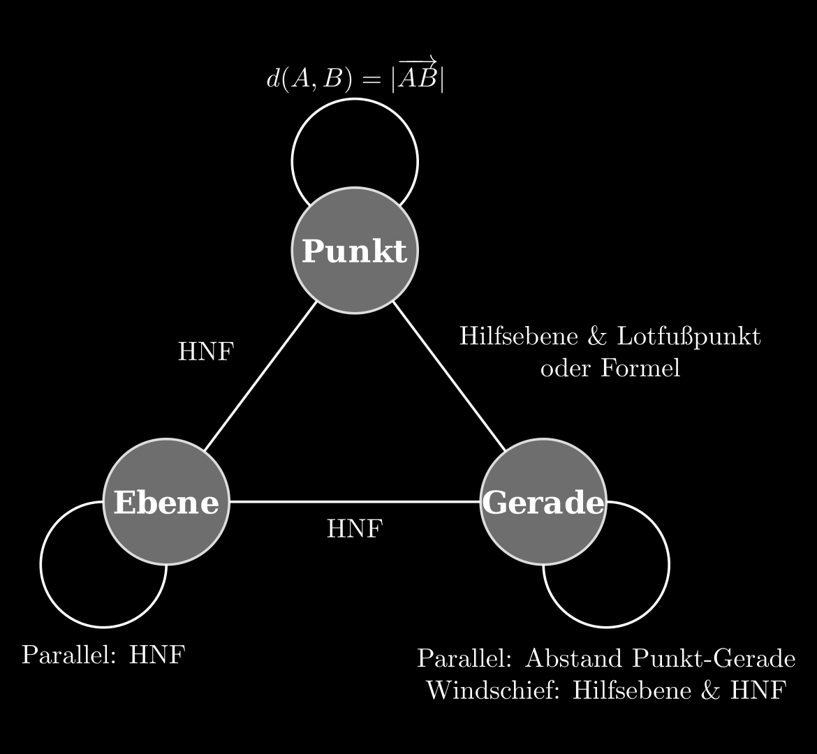
Abstandsberechnungen (Übersicht) 💡
Hesse’sche Normal(en)form (HNF) 💡
Eine Ebenengleichung E : ( x ⃗ − p ⃗ ) ∘ n ⃗ 0 = 0 E: (\vec x - \vec p) \circ \vec n_0 = 0 E : ( x − p ) ∘ n 0 = 0 Hesse’sche Normal(en)form (HNF) von E E E n ⃗ 0 \vec n_0 n 0 Einheitsnormalenvektor .
Der Abstand d ( E , Q ) d(E, Q) d ( E , Q ) E E E Q Q Q
d ( E , Q ) = ∣ ( q ⃗ − p ⃗ ) ∘ n ⃗ 0 ∣ d(E, Q) = |(\vec q - \vec p)\circ\vec n_0| d ( E , Q ) = ∣ ( q − p ) ∘ n 0 ∣ 💡
Für die Koordinatengleichung von E : a 1 x 1 + a 2 x 2 + a 3 x 3 = b E:a_1x_1+a_2x_2+a_3x_3=b E : a 1 x 1 + a 2 x 2 + a 3 x 3 = b
d ( E , Q ) = ∣ a 1 x 1 + a 2 x 2 + a 3 x 3 − b ∣ a 1 2 + a 2 2 + a 3 2 d(E, Q) = \frac {
|a_1x_1+a_2x_2+a_3x_3-b|
}{
\sqrt{{a_1}^2+{a_2}^2+{a_3}^2}
} d ( E , Q ) = a 1 2 + a 2 2 + a 3 2 ∣ a 1 x 1 + a 2 x 2 + a 3 x 3 − b ∣ Beispiele Normalenform:
E : [ x ⃗ − ( 9 − 8 6 ) ] ∘ ( 2 2 1 ) = 0 P ( 1 ∣ − 1 ∣ 0 ) E:
\left[
\vec x
-
\left(\begin{matrix}
9 \\ -8 \\ 6
\end{matrix}\right)
\right]
\circ
\left(\begin{matrix}
2 \\ 2 \\ 1
\end{matrix}
\right)
= 0
\qquad
P(1 \, | \, {-1} \, | \, 0) E : x − 9 − 8 6 ∘ 2 2 1 = 0 P ( 1 ∣ − 1 ∣ 0 ) d ( E , P ) = ∣ ( 0 − 1 1 ) − ( 9 − 8 6 ) ∘ ( 2 2 1 ) ∣ ⋅ 1 3 ⏟ n ⃗ 0 = ∣ ( − 9 7 − 5 ) ∘ ( 2 2 1 ) ∣ ⋅ 1 3 = 9 ⋅ 1 3 = 3 d(E, P) = \left|
\left(\begin{matrix}
0 \\ -1 \\ 1
\end{matrix}\right)
-
\left(\begin{matrix}
9 \\ -8 \\ 6
\end{matrix}\right)
\circ
\right.
\underbrace{
\left.
\left(\begin{matrix}
2 \\ 2 \\ 1
\end{matrix}\right)
\right|
\cdot\frac13
}_{\vec n_0} =
\left|
\left(\begin{matrix}
-9 \\ 7 \\ -5
\end{matrix}\right)
\circ
\left(\begin{matrix}
2 \\ 2 \\ 1
\end{matrix}\right)
\right|
\cdot\frac13
=
9 \cdot \frac 13 =3 d ( E , P ) = 0 − 1 1 − 9 − 8 6 ∘ n 0 2 2 1 ⋅ 3 1 = − 9 7 − 5 ∘ 2 2 1 ⋅ 3 1 = 9 ⋅ 3 1 = 3 Koordinatenform:
F : 2 x 1 − 4 x 2 + 4 x 3 = 2 Q ( 4 ∣ 2 ∣ 5 ) F: 2x_1-4x_2+4x_3 = 2 \qquad
Q(4 \, | \, 2 \, | \, 5) F : 2 x 1 − 4 x 2 + 4 x 3 = 2 Q ( 4 ∣ 2 ∣ 5 ) d ( F , Q ) = ∣ 2 ⋅ 4 − 4 ⋅ 2 + 4 ⋅ 5 − 2 ∣ 2 2 + 4 2 + 4 2 = ∣ 18 ∣ 36 = 3 d(F,Q) = \frac{
|2 \cdot 4 - 4 \cdot 2 +
4 \cdot 5 - 2|
}{
\sqrt{2^2+4^2+4^2}
}
=
\frac{|18|}{\sqrt{36}}
=
3 d ( F , Q ) = 2 2 + 4 2 + 4 2 ∣2 ⋅ 4 − 4 ⋅ 2 + 4 ⋅ 5 − 2∣ = 36 ∣18∣ = 3 Abstand Punkt-Ebene 💡
Unter dem Abstand d d d P P P E E E P P P E E E
Beispiel E : x 1 + 8 x 2 − 4 x 3 = 25 P ( 2 ∣ 0 ∣ 1 ) E: x_1 + 8x_2 -4x_3 = 25 \qquad
P(2 \, | \, 0 \, | \, 1) E : x 1 + 8 x 2 − 4 x 3 = 25 P ( 2 ∣ 0 ∣ 1 ) Variante 1: HNF d ( E , P ) = ∣ 2 − 4 − 25 ∣ 1 2 + 8 2 + 4 2 = ∣ − 27 ∣ 81 = 27 9 = 3 d(E, P) = \frac{
|2-4-25|
}{
\sqrt{1^2+8^2+4^2}
}
=
\frac{|{-27}|}{\sqrt{81}}
=
\frac{27}{9}=3 d ( E , P ) = 1 2 + 8 2 + 4 2 ∣2 − 4 − 25∣ = 81 ∣ − 27 ∣ = 9 27 = 3 Variante 2: Durchstoßpunkt Hilfsgerade g durch P in Richtung des Normalenvektors g : x ⃗ = ( 2 0 1 ) + r ⋅ ( 1 8 − 4 ) \text{Hilfsgerade }g \text{ durch }P \text{ in Richtung des Normalenvektors} \\
g: \vec x =
\left(\begin{matrix}
2 \\ 0 \\ 1
\end{matrix}\right)
+ r \cdot \left(\begin{matrix}
1 \\ 8 \\ -4
\end{matrix}\right) Hilfsgerade g durch P in Richtung des Normalenvektors g : x = 2 0 1 + r ⋅ 1 8 − 4 E & g schneiden um Lotfußpunkt zu bestimmen 2 + r + 8 ⋅ 8 r − 4 ⋅ ( 1 − 4 r ) = 25 ⇒ r = 1 3 ⇒ F ( 7 3 ∣ 8 3 ∣ − 1 3 ) E \text{ \& } g \text{ schneiden um Lotfußpunkt zu bestimmen} \\
\begin{align*}
2+r + 8 \cdot 8r -
4 \cdot (1-4r) &= 25
\\
\Rightarrow r &= \frac13
\end{align*}
\\\Rightarrow
F\left(
\frac73 \, \left| \,
\frac83 \, \right|
{-\frac13}
\right) E & g schneiden um Lotfußpunkt zu bestimmen 2 + r + 8 ⋅ 8 r − 4 ⋅ ( 1 − 4 r ) ⇒ r = 25 = 3 1 ⇒ F ( 3 7 3 8 − 3 1 ) d ( E , P ) = d ( F , P ) = ∣ F R → ∣ = ∣ ( 2 0 1 ) − ( 7 3 8 3 − 1 3 ) ∣ = ( 1 3 ) 2 + ( 8 3 ) 2 + ( 4 3 ) 2 = 9 = 3 \begin{align*}
d(E,P) = d(F,P) =
|\overrightarrow{FR}| &=
\left|
\left(\begin{matrix}
2 \\ 0 \\ 1
\end{matrix}\right)
-
\left(\begin{matrix}
\frac73 \\ \frac83 \\ -\frac13
\end{matrix}\right)
\right|
\\
&=\sqrt{
\left(\frac13\right)^2 +
\left(\frac83\right)^2 +
\left(\frac43\right)^2
}
=
\sqrt9 = 3
\end{align*} d ( E , P ) = d ( F , P ) = ∣ FR ∣ = 2 0 1 − 3 7 3 8 − 3 1 = ( 3 1 ) 2 + ( 3 8 ) 2 + ( 3 4 ) 2 = 9 = 3 Abstand Punkt-Gerade 💡
Algorithmus Stelle Hilfsebene H H H P P P g g g Erhalte Punkt F F F g g g H H H d ( R , g ) = ∣ F R → ∣ d(R, g) = |\overrightarrow{FR}| d ( R , g ) = ∣ FR ∣ 💡
Formel Für den Abstand eines Punktes R R R g : x ⃗ = p ⃗ + s ⋅ u ⃗ g: \vec x = \vec p + s \cdot \vec u g : x = p + s ⋅ u
d ( R , g ) = ∣ P R → × u ⃗ 0 ∣ d(R, g) = |\overrightarrow{PR} \times \vec u_0| d ( R , g ) = ∣ PR × u 0 ∣ Beispiel g : x ⃗ = ( 4 3 1 ) + s ⋅ ( 2 1 − 2 ) R ( 2 ∣ − 3 ∣ 5 ) g: \vec x =
\left(\begin{matrix}
4 \\ 3 \\ 1
\end{matrix}\right)
+ s \cdot
\left(\begin{matrix}
2 \\ 1 \\ -2
\end{matrix}\right)
\qquad
R(2 \, | {-3} \, | \,5) g : x = 4 3 1 + s ⋅ 2 1 − 2 R ( 2 ∣ − 3 ∣ 5 ) Variante 1: Algorithmus 1. Hilfsebene aufstellen ⇒ H : 2 x 1 + x 2 − 2 x 3 = − 9 NR: 2 ⋅ 2 + ( − 3 ) − 2 ⋅ 5 = − 9 \text{1. Hilfsebene aufstellen} \\
\Rightarrow H: 2x_1 +x_2 -2x_3 = -9
\qquad
\text{NR: }
2\cdot2 + (-3) - 2 \cdot 5 = -9
1. Hilfsebene aufstellen ⇒ H : 2 x 1 + x 2 − 2 x 3 = − 9 NR: 2 ⋅ 2 + ( − 3 ) − 2 ⋅ 5 = − 9 2. Schnittpunkt bestimmen 2 ⋅ ( 4 + 2 s ) + 3 + s − 2 ⋅ ( 1 − 2 s ) = − 9 9 + 9 s = − 9 ∣ − 9 ∣ : 9 s = − 2 ⇒ F ( 0 ∣ 1 ∣ 5 ) \text{2. Schnittpunkt bestimmen}\\
\begin{align*}
2 \cdot (4+2s) + 3 + s -
2 \cdot (1 - 2s)
&= -9 \\
9+9s &= -9 \quad |-9 \ |:9 \\
s &= -2
\end{align*}
\\
\Rightarrow
F(0 \, | \, 1 \, | \,5) 2. Schnittpunkt bestimmen 2 ⋅ ( 4 + 2 s ) + 3 + s − 2 ⋅ ( 1 − 2 s ) 9 + 9 s s = − 9 = − 9 ∣ − 9 ∣ : 9 = − 2 ⇒ F ( 0 ∣ 1 ∣ 5 ) 3. Abstand berechnen d ( R , g ) = d ( R , F ) = ∣ R F → ∣ = 2 2 + 4 2 + 0 2 = 20 \text{3. Abstand berechnen}\\
d(R, g) = d(R, F) = |\overrightarrow{RF}| =
\sqrt{2^2+4^2+0^2}=\sqrt{20} 3. Abstand berechnen d ( R , g ) = d ( R , F ) = ∣ RF ∣ = 2 2 + 4 2 + 0 2 = 20 Variante 2: Formel R P → = ( 2 6 − 4 ) ∣ u ⃗ ∣ = 3 ⇒ u ⃗ 0 = 1 3 ⋅ ( 2 1 − 2 ) \overrightarrow{RP} =
\left(\begin{matrix}
2 \\ 6 \\ -4
\end{matrix}\right)
\qquad
|\vec u| = 3
\ \ \Rightarrow \ \
\vec u_0 =
\frac1{3} \cdot
\left(\begin{matrix}
2 \\ 1 \\ -2
\end{matrix}\right) RP = 2 6 − 4 ∣ u ∣ = 3 ⇒ u 0 = 3 1 ⋅ 2 1 − 2 d ( R , g ) = ∣ R P → × u ⃗ 0 ∣ = ∣ ( 2 6 − 4 ) × ( 2 1 − 2 ) ∣ ⋅ 1 3 ⏟ u ⃗ 0 = ∣ ( − 8 − 4 − 10 ) ∣ ⋅ 1 3 = 180 ⋅ 1 9 = 20 \begin{align*}
d(R, g) =
|\overrightarrow{RP}
\times \vec u_0| &=
\left|
\left(\begin{matrix}
2 \\ 6 \\ -4
\end{matrix}\right)
\times
\right.
\underbrace{
\left.
\left(\begin{matrix}
2 \\ 1 \\ -2
\end{matrix}\right)
\right|
\cdot \frac 13
}_{\vec u_0}\\
&=
\left|
\left(\begin{matrix}
-8 \\ -4 \\ -10
\end{matrix}\right)
\right|
\cdot \frac 13
=\sqrt{180}\cdot\sqrt{\frac19}
=\sqrt{20}
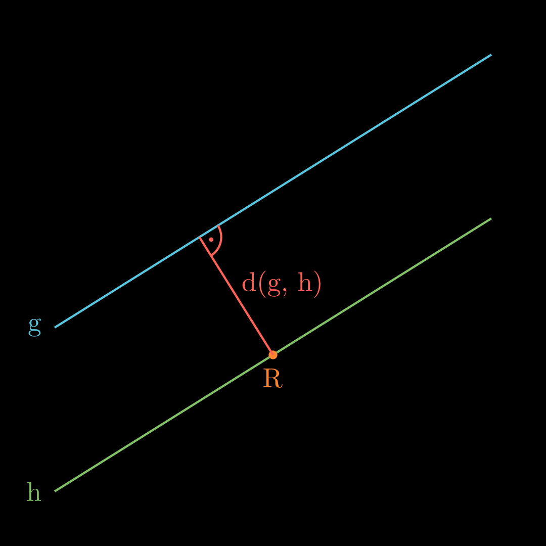
\end{align*} d ( R , g ) = ∣ RP × u 0 ∣ = 2 6 − 4 × u 0 2 1 − 2 ⋅ 3 1 = − 8 − 4 − 10 ⋅ 3 1 = 180 ⋅ 9 1 = 20 Abstand Gerade-Gerade (Parallel) 💡
Um den Abstand zwei paralleler Geraden g g g h h h R R R h h h g g g
d ( g , h ) = d ( g , R ) d(g, h) = d(g,R) d ( g , h ) = d ( g , R ) Beispiel Siehe Beispiel Abstand Punkt-Gerade.
Abstand Gerade-Gerade (Windschief) 💡
Gegeben sind die Geraden g : x ⃗ = p ⃗ + r ⋅ u ⃗ g: \vec x = \vec p + r \cdot \vec u g : x = p + r ⋅ u h : x ⃗ = q ⃗ + s ⋅ v ⃗ h: \vec x = \vec q + s \cdot \vec v h : x = q + s ⋅ v
Stelle eine Hilfsebene E E E n ⃗ = u ⃗ × v ⃗ \vec n = \vec u \times \vec v n = u × v P P P E E E h h h g g g d ( g , h ) = d ( E , h ) = d ( E , Q ) ⏟ HNF d(g, h) = d(E, h) = \underbrace{d(E, Q)}_{\text{HNF}} d ( g , h ) = d ( E , h ) = HNF d ( E , Q ) ODER
d ( g , h ) = ∣ ( q ⃗ − p ⃗ ) ∘ n ⃗ 0 ∣ d(g, h) = \left | (\vec q - \vec p) \circ \vec n_0 \right | d ( g , h ) = ∣ ( q − p ) ∘ n 0 ∣
Beispiel g : x ⃗ = ( 9 − 8 6 ) + r ⋅ ( 2 − 3 2 ) h : x ⃗ = ( 6 5 4 ) + s ⋅ ( 1 − 1 0 ) g: \vec x =
\left(\begin{matrix}
9 \\ -8 \\ 6
\end{matrix}\right)
+ r \cdot
\left(\begin{matrix}
2 \\ -3 \\ 2
\end{matrix}\right)
\qquad
h: \vec x =
\left(\begin{matrix}
6 \\ 5 \\ 4
\end{matrix}\right)
+ s \cdot
\left(\begin{matrix}
1 \\ -1 \\ 0
\end{matrix}\right) g : x = 9 − 8 6 + r ⋅ 2 − 3 2 h : x = 6 5 4 + s ⋅ 1 − 1 0 n ⃗ = ( 2 − 3 2 ) × ( 1 − 1 0 ) = ( 2 2 1 ) ∣ n ⃗ ∣ = 3 \vec n =
\left(\begin{matrix}
2 \\ -3 \\ 2
\end{matrix}\right)
\times
\left(\begin{matrix}
1 \\ -1 \\ 0
\end{matrix}\right)
=
\left(\begin{matrix}
2 \\ 2 \\ 1
\end{matrix}\right)
\qquad
|\vec n| =3 n = 2 − 3 2 × 1 − 1 0 = 2 2 1 ∣ n ∣ = 3 d ( E , Q ) = ∣ ( 6 5 4 ) − ( 9 − 8 6 ) ∘ ( 2 2 1 ) ∣ ⋅ 1 3 ⏟ n ⃗ 0 = ∣ ( − 3 13 − 2 ) ∘ ( 2 2 1 ) ∣ ⋅ 1 3 = 18 ⋅ 1 3 = 6 d(E, Q) = \left|
\left(\begin{matrix}
6 \\ 5 \\ 4
\end{matrix}\right)
-
\left(\begin{matrix}
9 \\ -8 \\ 6
\end{matrix}\right)
\circ
\right.
\underbrace{
\left.
\left(\begin{matrix}
2 \\ 2 \\ 1
\end{matrix}\right)
\right|
\cdot\frac13
}_{\vec n_0} =
\left|
\left(\begin{matrix}
-3 \\ 13 \\ -2
\end{matrix}\right)
\circ
\left(\begin{matrix}
2 \\ 2 \\ 1
\end{matrix}\right)
\right|
\cdot\frac13
=
18 \cdot \frac 13 = 6 d ( E , Q ) = 6 5 4 − 9 − 8 6 ∘ n 0 2 2 1 ⋅ 3 1 = − 3 13 − 2 ∘ 2 2 1 ⋅ 3 1 = 18 ⋅ 3 1 = 6 ODER
d ( g , h ) = ∣ ( ( 6 5 4 ) − ( 9 − 8 6 ) ) ∘ 1 3 ⋅ ( 2 2 1 ) ⏟ n ⃗ 0 ∣ = ∣ ( − 3 13 − 2 ) ∘ ( 2 3 2 3 1 3 ) ∣ = 6 d(g, h) = \left|
\left(
\left(\begin{matrix}
6 \\ 5 \\ 4
\end{matrix}\right)
-
\left(\begin{matrix}
9 \\ -8 \\ 6
\end{matrix}\right)
\right)
\circ
\underbrace {
\frac13 \cdot
\left(\begin{matrix}
2 \\ 2 \\ 1
\end{matrix}\right)
}_{\vec n_0}
\right|
=
\left|
\left(\begin{matrix}
-3 \\ 13 \\ -2
\end{matrix}\right)
\circ
\left(\begin{matrix}
\frac23 \\ \frac23 \\ \frac13
\end{matrix}\right)
\right|
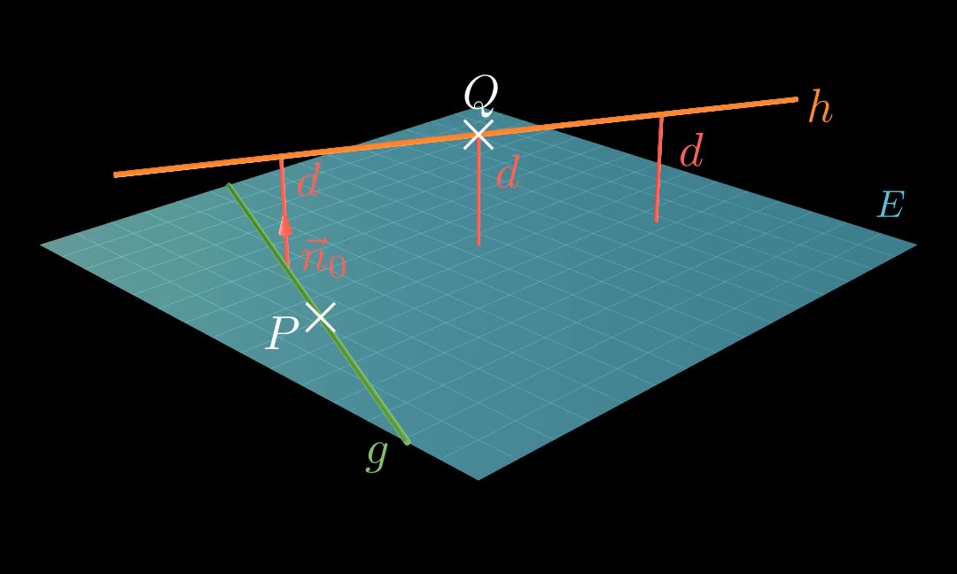
=6 d ( g , h ) = 6 5 4 − 9 − 8 6 ∘ n 0 3 1 ⋅ 2 2 1 = − 3 13 − 2 ∘ 3 2 3 2 3 1 = 6 Abstand Gerade-Ebene (Parallel) 💡
Um den Abstand der Ebene E E E g g g Q Q Q g g g
d ( E , g ) = d ( E , Q ) ⏟ HNF d(E, g) =
\underbrace{d(E, Q)}
_{\text{HNF}} d ( E , g ) = HNF d ( E , Q ) Beispiel E : x 1 + 2 x 2 − 2 x 3 = 4 g : x ⃗ = ( 4 2 1 ) + t ⋅ ( 0 1 1 ) E: x_1 + 2x_2 - 2x_3 = 4
\qquad
g: \vec x =
\left(\begin{matrix}
4 \\ 2 \\ 1
\end{matrix}\right)
+ t \cdot
\left(\begin{matrix}
0 \\ 1 \\ 1
\end{matrix}\right) E : x 1 + 2 x 2 − 2 x 3 = 4 g : x = 4 2 1 + t ⋅ 0 1 1 d ( E , g ) = d ( E , ( 4 ∣ 2 ∣ 1 ) ) = ∣ 4 + 4 − 2 − 4 ∣ 3 = 2 3 d(E, g) =
d(E, (4 \, | \, 2 \, | \, 1)) =
\frac{|4+4-2-4|}{3} = \frac23 d ( E , g ) = d ( E , ( 4 ∣ 2 ∣ 1 )) = 3 ∣4 + 4 − 2 − 4∣ = 3 2 Abstand Ebene-Ebene (Parallel) 💡
Um den Abstand der parallelen Ebenen E E E F F F P P P F F F
d ( E , F ) = d ( E , P ) ⏟ HNF d(E, F) =
\underbrace{d(E, P)}
_{\text{HNF}} d ( E , F ) = HNF d ( E , P ) Beispiel E : x 1 + 2 x 2 − 2 x 3 = 4 F : 3 x 1 + 6 x 2 − 6 x 3 = 21 ⇒ P ( 7 ∣ 0 ∣ 0 ) \begin{align*}
E: x_1 + 2x_2 - 2x_3 = 4
\qquad
&F: 3x_1 + 6x_2 - 6x_3 = 21
\\&\quad\Rightarrow
P(7 \, | \, 0 \, | \, 0)
\end{align*} E : x 1 + 2 x 2 − 2 x 3 = 4 F : 3 x 1 + 6 x 2 − 6 x 3 = 21 ⇒ P ( 7 ∣ 0 ∣ 0 ) d ( E , F ) = d ( E , P ) = ∣ 7 − 4 ∣ 3 = 1 d(E, F) = d(E, P) =
\frac{|7-4|}{3} = 1 d ( E , F ) = d ( E , P ) = 3 ∣7 − 4∣ = 1 Gemeinsames Lot windschiefer Geraden bestimmen 💡
Um das gemeinsame Lot zweier windschiefer Geraden g g g h h h P P P g g g Q Q Q h h h P Q → \overrightarrow{PQ} PQ g g g h h h
Beispiel g : x ⃗ = ( 7 7 0 ) + r ⋅ ( 4 − 5 2 ) h : x ⃗ = ( 0 1 2 ) + s ⋅ ( 0 1 1 ) P r ( 7 + 4 r ∣ 7 − 5 r ∣ 2 r ) Q s ( 0 ∣ 1 + s ∣ 2 + s ) \begin{align*}
&g: \vec x =
\left(\begin{matrix}
7 \\ 7 \\ 0
\end{matrix}\right)
+ r \cdot
\left(\begin{matrix}
4 \\ -5 \\ 2
\end{matrix}\right)
\qquad
h: \vec x &=
\left(\begin{matrix}
0 \\ 1 \\ 2
\end{matrix}\right)
+ s \cdot
\left(\begin{matrix}
0 \\ 1 \\ 1
\end{matrix}\right)
\\
&P_r(7+4r \, | \, 7-5r \, | \, 2r)
&Q_s(0 \, | \, 1+s \, | \, 2+s)
\end{align*} g : x = 7 7 0 + r ⋅ 4 − 5 2 h : x P r ( 7 + 4 r ∣ 7 − 5 r ∣ 2 r ) = 0 1 2 + s ⋅ 0 1 1 Q s ( 0 ∣ 1 + s ∣ 2 + s ) Suche t & s , sodass P r Q s → ⊥ g & P r Q s → ⊥ h ( 7 + 4 r 7 − 5 r − ( 1 + s ) 2 s − ( 2 + s ) ) ∘ ( 4 − 5 2 ) = 0 28 + 16 r − 35 + 25 r + 5 + 5 s + 4 r − 4 + 2 s = 0 − 6 + 45 r + 3 s = 0 ⇒ s = 2 − 15 r ⇒ In ander gleichung einsetzen ( 7 + 4 r 7 − 5 r − ( 1 + s ) 2 r − ( 2 + s ) ) ∘ ( 0 1 1 ) = 0 7 − 5 r − 1 − s + 2 r − 2 − s = 0 4 − 3 r − 2 s = 0 ∣ s = 2 − 15 r 4 − 3 r − 4 + 30 r = 0 r = 0 ⇒ s = 2 G ( 7 ∣ 7 ∣ 0 ) H ( 0 ∣ 3 ∣ 4 ) \text{Suche } t \ \& \ s
\text{, sodass }
\overrightarrow{P_rQ_s} \perp g
\ \& \
\overrightarrow{P_rQ_s} \perp h
\\
\begin{align*}
\left(\begin{matrix}
7+4r \\ 7-5r-(1+s) \\ 2s-(2+s)
\end{matrix}\right)
\circ
\left(\begin{matrix}
4 \\ -5 \\ 2
\end{matrix}\right)
&= 0
\\
28+16r-35+25r+5+5s+4r-4+2s &= 0
\\
-6 + 45r + 3s &= 0
\\
\Rightarrow
s = 2-&15r
\\
\xRightarrow {\text{In ander gleichung einsetzen}}
\end{align*}
\qquad
\begin{align*}
\left(\begin{matrix}
7+4r \\ 7-5r-(1+s) \\ 2r-(2+s)
\end{matrix}\right)
\circ
\left(\begin{matrix}
0 \\ 1 \\ 1
\end{matrix}\right)
&= 0
\\
7-5r-1-s+2r-2-s &=0
\\
4-3r-2s &=0
\quad |\ s =2-15r
\\
4-3r-4+30r &= 0
\\
r &= 0
\\
\Rightarrow &s=2
\end{align*}
\\
\boxed{
G(\, 7 \, | \, 7 \, | \, 0)
\quad
H(\, 0 \, | \, 3 \, | \, 4)
} Suche t & s , sodass P r Q s ⊥ g & P r Q s ⊥ h 7 + 4 r 7 − 5 r − ( 1 + s ) 2 s − ( 2 + s ) ∘ 4 − 5 2 28 + 16 r − 35 + 25 r + 5 + 5 s + 4 r − 4 + 2 s − 6 + 45 r + 3 s ⇒ s = 2 − In ander gleichung einsetzen = 0 = 0 = 0 15 r 7 + 4 r 7 − 5 r − ( 1 + s ) 2 r − ( 2 + s ) ∘ 0 1 1 7 − 5 r − 1 − s + 2 r − 2 − s 4 − 3 r − 2 s 4 − 3 r − 4 + 30 r r ⇒ = 0 = 0 = 0 ∣ s = 2 − 15 r = 0 = 0 s = 2 G ( 7 ∣ 7 ∣ 0 ) H ( 0 ∣ 3 ∣ 4 ) 💬
Wenn die Fragestellung nach den Lotfußpunkten fragt, reicht es die Punkte G G G H H H G G G H H H
Winkel zwischen Vektoren 💡
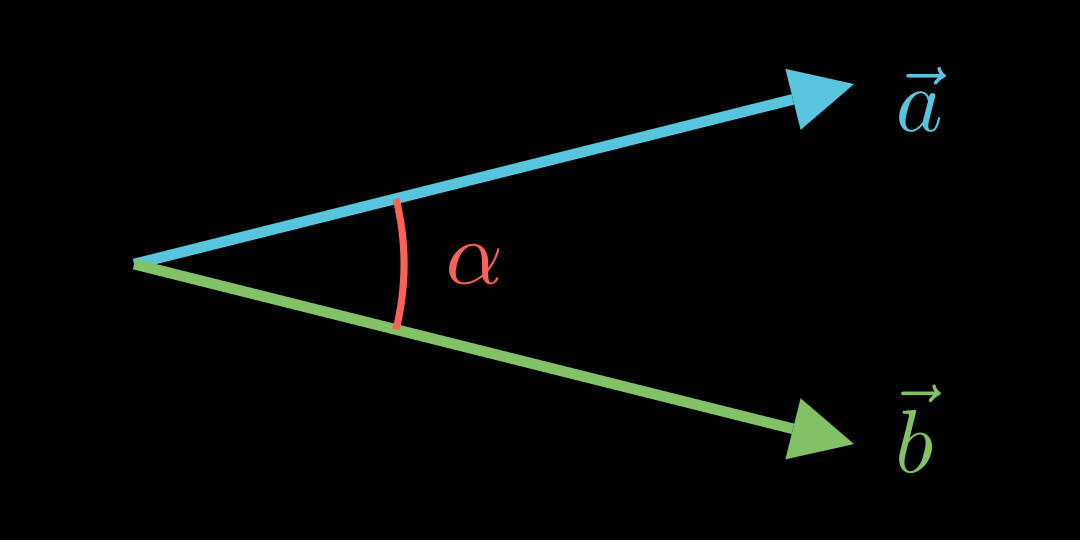
Für den Winkel α \alpha α a ⃗ \vec a a b ⃗ \vec b b
cos ( α ) = a ⃗ ∘ b ⃗ ∣ a ⃗ ∣ ⋅ ∣ b ⃗ ∣ \cos(\alpha)=\frac{
\vec a \circ \vec b
}{
|\vec a| \cdot |\vec b|} cos ( α ) = ∣ a ∣ ⋅ ∣ b ∣ a ∘ b Beispiel a ⃗ = ( − 2 3 1 ) b ⃗ = ( 4 0 3 ) \vec a =
\left(\begin{matrix}
-2 \\ 3 \\ 1
\end{matrix}\right)
\qquad
\vec b =
\left(\begin{matrix}
4 \\ 0 \\ 3
\end{matrix}\right) a = − 2 3 1 b = 4 0 3 ∣ a ⃗ ∣ = 14 ∣ b ⃗ ∣ = 5 cos ( α ) = ( − 2 3 1 ) ∘ ( 4 0 3 ) 14 ⋅ 5 cos ( α ) = − 5 14 ⋅ 5 α = cos − 1 ( − 1 14 ) ⏟ DEGREE! ≈ 105 , 5 ° |\vec a| = \sqrt{14}
\qquad
|\vec b| = 5
\\
\begin{align*}
\\
\cos(\alpha) &= \frac{
\left(\begin{matrix}
-2 \\ 3 \\ 1
\end{matrix}\right)
\circ
\left(\begin{matrix}
4 \\ 0 \\ 3
\end{matrix}\right)
}{
\sqrt{14} \cdot 5
}
\\
\cos(\alpha) &= \frac{
-5}{
\sqrt{14} \cdot 5
}
\\
\alpha &=
\underbrace{
\cos^{-1}\left(-\frac{1}{\sqrt{14}}\right)
}_{
\color{red} \text{DEGREE!}
}
\boxed{\approx 105{,}5°}
\end{align*} ∣ a ∣ = 14 ∣ b ∣ = 5 cos ( α ) cos ( α ) α = 14 ⋅ 5 − 2 3 1 ∘ 4 0 3 = 14 ⋅ 5 − 5 = DEGREE! cos − 1 ( − 14 1 ) ≈ 105 , 5° Schnittwinkel Gerade-Gerade 💡
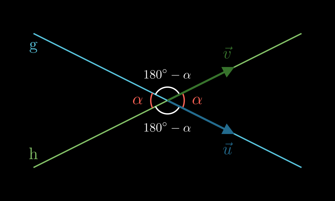
Für den Schnittwinkel zwischen zwei Geraden g g g h h h u ⃗ \vec u u v ⃗ \vec v v
cos ( α ) = ∣ u ⃗ ∘ v ⃗ ∣ ∣ u ⃗ ∣ ⋅ ∣ v ⃗ ∣ \cos(\alpha) = \frac{
|\vec u \circ \vec v|}{
|\vec u| \cdot |\vec v|} cos ( α ) = ∣ u ∣ ⋅ ∣ v ∣ ∣ u ∘ v ∣ Beispiel u ⃗ = ( − 2 3 1 ) v ⃗ = ( 4 0 3 ) \vec u =
\left(\begin{matrix}
-2 \\ 3 \\ 1
\end{matrix}\right)
\qquad
\vec v =
\left(\begin{matrix}
4 \\ 0 \\ 3
\end{matrix}\right) u = − 2 3 1 v = 4 0 3 ∣ u ⃗ ∣ = 14 ∣ v ⃗ ∣ = 5 cos ( α ) = ∣ ( − 2 3 1 ) ∘ ( 4 0 3 ) ∣ 14 ⋅ 5 cos ( α ) = ∣ − 5 ∣ 14 ⋅ 5 α = cos − 1 ( 1 14 ) ⏟ DEGREE! ≈ 74 , 5 ° |\vec u| = \sqrt{14}
\qquad
|\vec v| = 5
\\
\begin{align*}
\\
\cos(\alpha) &= \frac{
\left|
\left(\begin{matrix}
-2 \\ 3 \\ 1
\end{matrix}\right)
\circ
\left(\begin{matrix}
4 \\ 0 \\ 3
\end{matrix}\right)
\right|
}{
\sqrt{14} \cdot 5
}
\\
\cos(\alpha) &= \frac{
|-5|}{
\sqrt{14} \cdot 5
}
\\
\alpha &=
\underbrace{
\cos^{-1}\left(\frac{1}{\sqrt{14}}\right)
}_{
\color{red} \text{DEGREE!}
}
\boxed{\approx 74{,}5°}
\end{align*} ∣ u ∣ = 14 ∣ v ∣ = 5 cos ( α ) cos ( α ) α = 14 ⋅ 5 − 2 3 1 ∘ 4 0 3 = 14 ⋅ 5 ∣ − 5∣ = DEGREE! cos − 1 ( 14 1 ) ≈ 74 , 5° Schnittwinkel Ebene-Ebene 💡
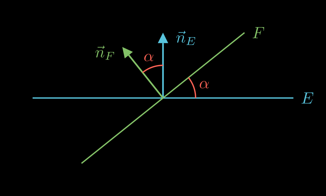
Für den Schnittwinkel zwischen zwei Ebenen E E E F F F n ⃗ E \vec n_E n E n ⃗ f \vec n_f n f
cos ( α ) = ∣ n ⃗ E ∘ n ⃗ F ∣ ∣ n ⃗ E ∣ ⋅ ∣ n ⃗ F ∣ \cos(\alpha) = \frac{
|\vec n_E \circ \vec n_F|}{
|\vec n_E| \cdot |\vec n_F|} cos ( α ) = ∣ n E ∣ ⋅ ∣ n F ∣ ∣ n E ∘ n F ∣ Beispiel Siehe Beispiel Schnittwinkel Gerade-Gerade.
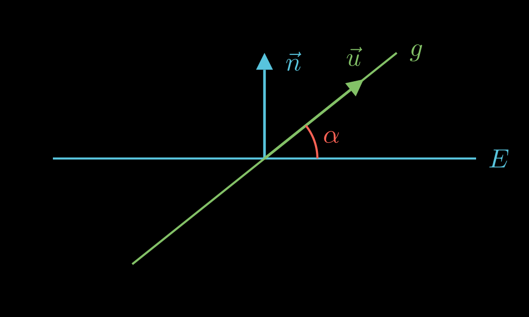
Schnittwinkel Gerade-Ebene 💡
Für den Schnittwinkel zwischen einer Geraden mit Richtungsvektoren u ⃗ \vec u u n ⃗ \vec n n
sin ( α ) = ∣ u ⃗ ∘ n ⃗ ∣ ∣ u ⃗ ∣ ⋅ ∣ n ⃗ ∣ {\color{red}\sin(\alpha)} = \frac{
|\vec u \circ \vec n|}{
|\vec u| \cdot |\vec n|} s i n ( α ) = ∣ u ∣ ⋅ ∣ n ∣ ∣ u ∘ n ∣ u ⃗ = ( 4 − 3 0 ) n ⃗ = ( 2 4 1 ) \vec u =
\left(\begin{matrix}
4 \\ -3 \\ 0
\end{matrix}\right)
\qquad
\vec n =
\left(\begin{matrix}
2 \\ 4 \\ 1
\end{matrix}\right) u = 4 − 3 0 n = 2 4 1 ∣ u ⃗ ∣ = 5 ∣ n ⃗ ∣ = 21 sin ( α ) = ∣ ( 4 − 3 0 ) ∘ ( 2 4 1 ) ∣ 5 ⋅ 21 sin ( α ) = ∣ − 4 ∣ 5 ⋅ 21 α = sin − 1 ( 4 5 ⋅ 21 ) ⏟ DEGREE! ≈ 10 , 1 ° |\vec u| = 5
\qquad
|\vec n| = \sqrt{21}
\\
\begin{align*}
\\
\sin(\alpha) &= \frac{
\left|
\left(\begin{matrix}
4 \\ -3 \\ 0
\end{matrix}\right)
\circ
\left(\begin{matrix}
2 \\ 4 \\ 1
\end{matrix}\right)
\right|
}{
5 \cdot \sqrt{21}
}
\\
\sin(\alpha) &= \frac{
|-4|}{
5 \cdot \sqrt{21}
}
\\
\alpha &=
\underbrace{
\sin^{-1}\left(\frac{4}{5 \cdot \sqrt{21}}\right)
}_{
\color{red} \text{DEGREE!}
}
\boxed{\approx 10{,}1°}
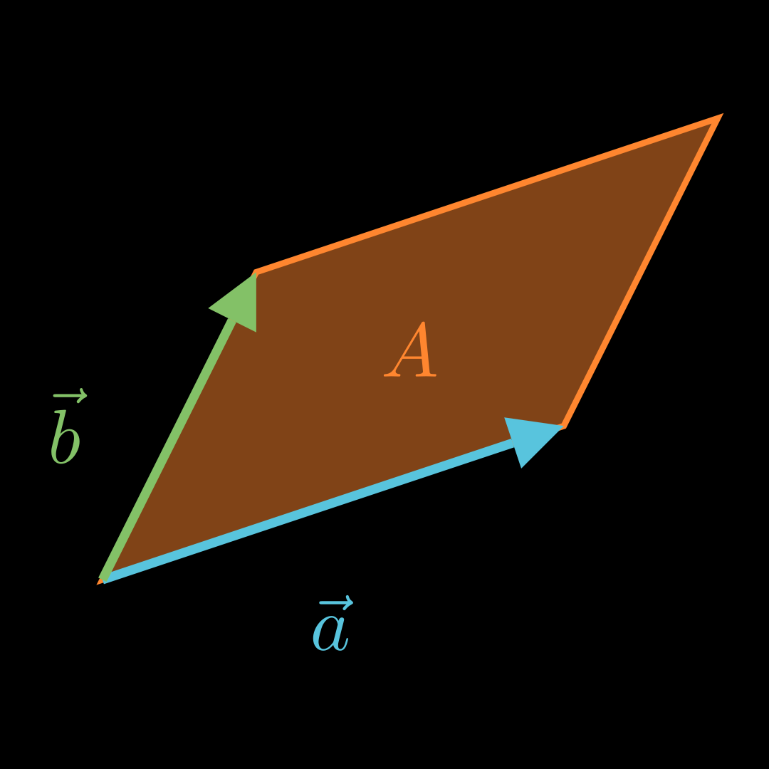
\end{align*} ∣ u ∣ = 5 ∣ n ∣ = 21 sin ( α ) sin ( α ) α = 5 ⋅ 21 4 − 3 0 ∘ 2 4 1 = 5 ⋅ 21 ∣ − 4∣ = DEGREE! sin − 1 ( 5 ⋅ 21 4 ) ≈ 10 , 1° Flächeninhalt Parallelogramm 💡
Für den Flächeninhalt A A A a ⃗ \vec a a b ⃗ \vec b b
A = ∣ a ⃗ × b ⃗ ∣ A=|\vec a \times \vec b| A = ∣ a × b ∣ Beispiel a ⃗ = ( 4 − 2 7 ) b ⃗ = ( 1 5 0 ) \vec a =
\left(\begin{matrix}
4 \\ -2 \\ 7
\end{matrix}\right)
\qquad
\vec b =
\left(\begin{matrix}
1 \\ 5 \\ 0
\end{matrix}\right) a = 4 − 2 7 b = 1 5 0 A = ∣ ( 4 − 2 7 ) × ( 1 5 0 ) ∣ = ∣ ( − 35 7 22 ) ∣ ≈ 41 , 93 A = \left|
\left(\begin{matrix}
4 \\ -2 \\ 7
\end{matrix}\right)
\times
\left(\begin{matrix}
1 \\ 5 \\ 0
\end{matrix}\right)
\right|
=
\left|
\left(\begin{matrix}
-35 \\ 7 \\ 22
\end{matrix}\right)
\right|
\approx
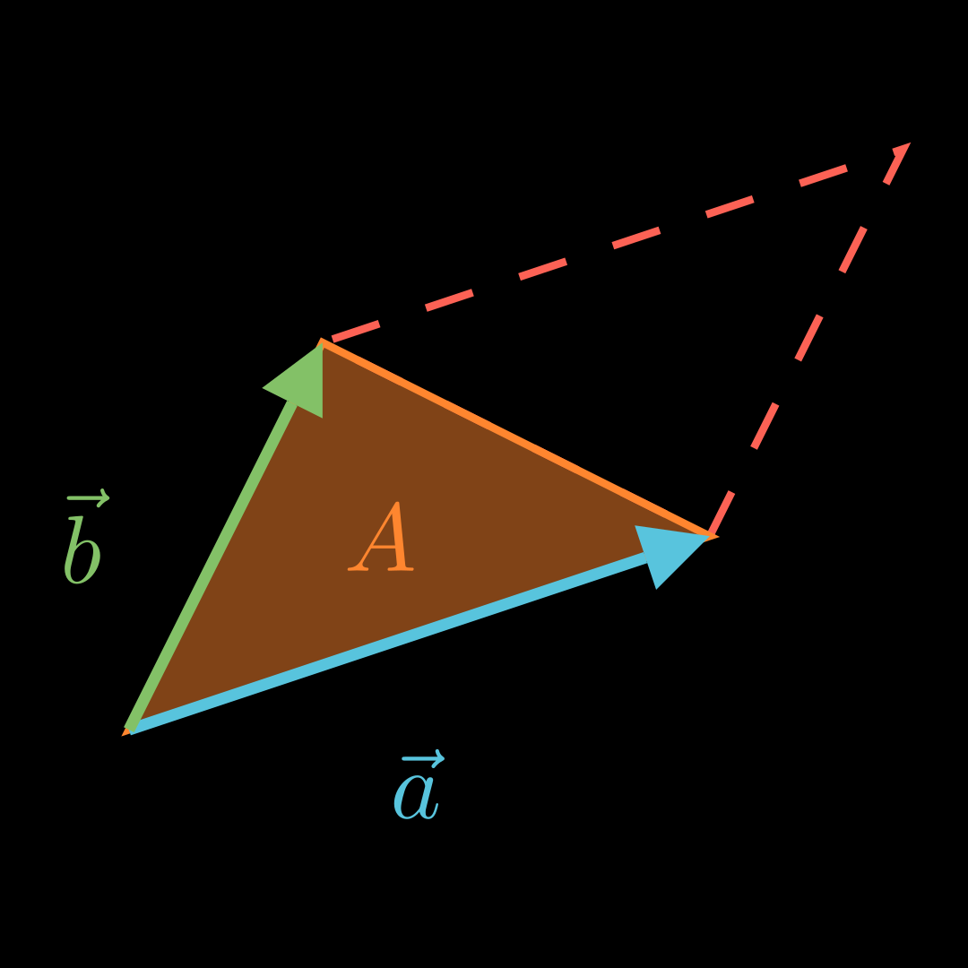
41{,}93 A = 4 − 2 7 × 1 5 0 = − 35 7 22 ≈ 41 , 93 Flächeninhalt Dreieck 💡
Für den Flächeninhalt A A A a ⃗ \vec a a b ⃗ \vec b b
A = 1 2 ⋅ ∣ a ⃗ × b ⃗ ∣ A = \frac12 \cdot
|\vec a \times \vec b| A = 2 1 ⋅ ∣ a × b ∣ Beispiel a ⃗ = ( 4 − 2 7 ) b ⃗ = ( 1 5 0 ) \vec a =
\left(\begin{matrix}
4 \\ -2 \\ 7
\end{matrix}\right)
\qquad
\vec b =
\left(\begin{matrix}
1 \\ 5 \\ 0
\end{matrix}\right) a = 4 − 2 7 b = 1 5 0 A = 1 2 ⋅ ∣ ( 4 − 2 7 ) × ( 1 5 0 ) ∣ = 1 2 ⋅ ∣ ( − 35 7 22 ) ∣ ≈ 1 2 ⋅ 41 , 93 = 20 , 965 A =
\frac12 \cdot
\left|
\left(\begin{matrix}
4 \\ -2 \\ 7
\end{matrix}\right)
\times
\left(\begin{matrix}
1 \\ 5 \\ 0
\end{matrix}\right)
\right|
=
\frac12 \cdot
\left|
\left(\begin{matrix}
-35 \\ 7 \\ 22
\end{matrix}\right)
\right|
\approx
\frac12 \cdot
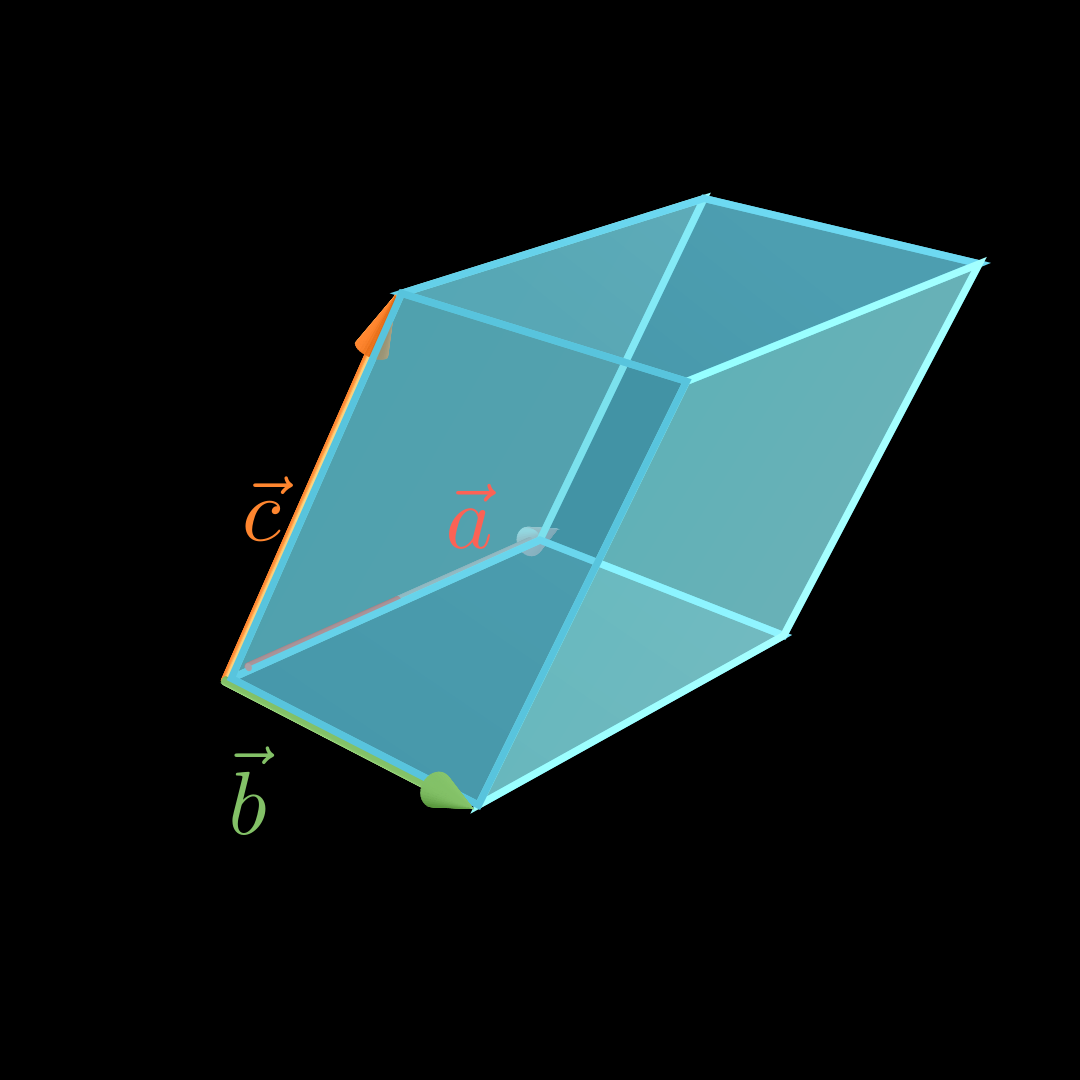
41{,}93 = 20{,}965 A = 2 1 ⋅ 4 − 2 7 × 1 5 0 = 2 1 ⋅ − 35 7 22 ≈ 2 1 ⋅ 41 , 93 = 20 , 965 Volumen Spat 💡
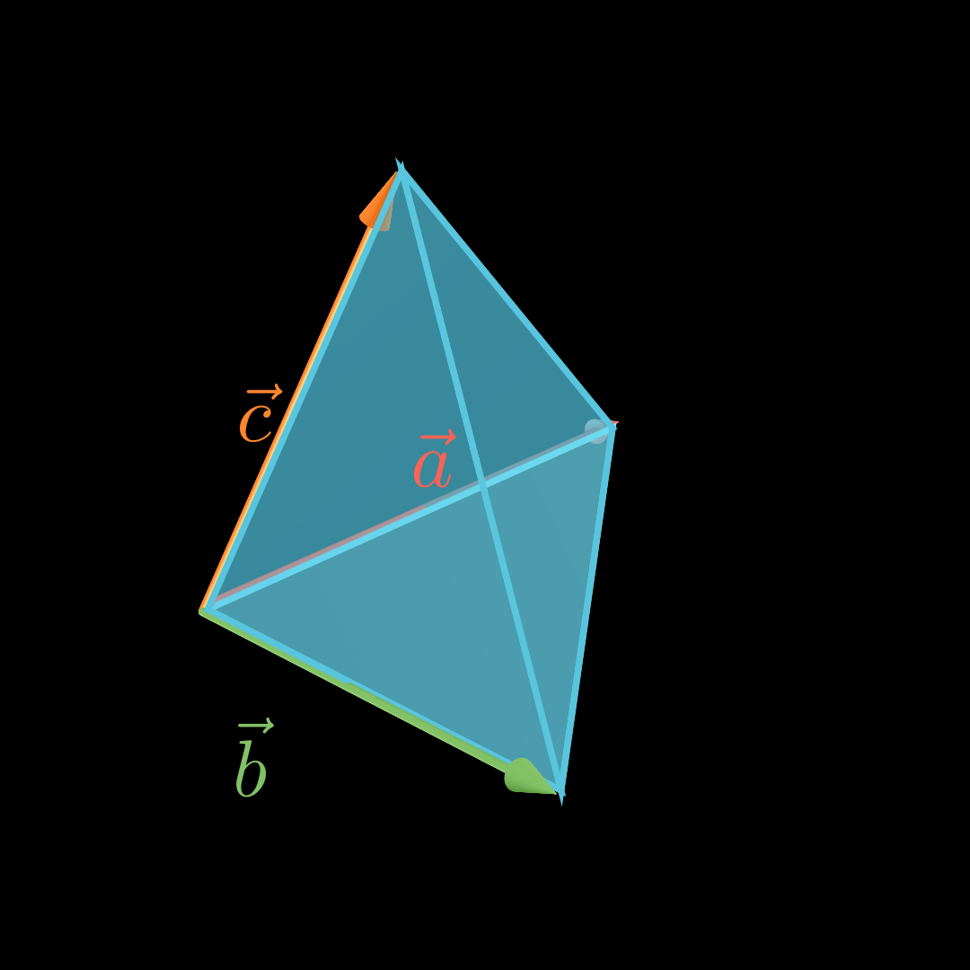
Für das Volumen V V V a ⃗ , b ⃗ \vec a, \vec b a , b c ⃗ \vec c c
V = ∣ ( a ⃗ × b ⃗ ) ∘ c ⃗ ∣ V =
|(\vec a \times \vec b)
\circ \vec c \, | V = ∣ ( a × b ) ∘ c ∣ Beispiel a ⃗ = ( − 4 2 0 ) b ⃗ = ( − 4 − 3 5 ) c ⃗ = ( − 2 0 10 ) \vec a =
\left(\begin{matrix}
-4 \\ 2 \\ 0
\end{matrix}\right)
\qquad
\vec b =
\left(\begin{matrix}
-4 \\ -3 \\ 5
\end{matrix}\right)
\qquad
\vec c =
\left(\begin{matrix}
-2 \\ 0 \\ 10
\end{matrix}\right) a = − 4 2 0 b = − 4 − 3 5 c = − 2 0 10 V = ∣ [ ( − 4 2 0 ) × ( − 4 − 3 5 ) ] ∘ ( − 2 0 10 ) ∣ = ∣ ( 10 20 20 ) ∘ ( − 2 0 10 ) ∣ = ∣ − 20 + 200 ∣ = 180 \begin{align*}
V &= \left|
\left[
\left(\begin{matrix}
-4 \\ 2 \\ 0
\end{matrix}\right)
\times
\left(\begin{matrix}
-4 \\ -3 \\ 5
\end{matrix}\right)
\right]
\circ
\left(\begin{matrix}
-2 \\ 0 \\ 10
\end{matrix}\right)
\right|
\\
&= \left|
\left(\begin{matrix}
10 \\ 20 \\ 20
\end{matrix}\right)
\circ
\left(\begin{matrix}
-2 \\ 0 \\ 10
\end{matrix}\right)
\right|
\\&=|{-20}+200|
\\&= 180
\end{align*} V = − 4 2 0 × − 4 − 3 5 ∘ − 2 0 10 = 10 20 20 ∘ − 2 0 10 = ∣ − 20 + 200∣ = 180 Volumen Pyramide mit viereckiger Grundfläche 💡
Für das Volumen V V V a ⃗ , b ⃗ \vec a, \vec b a , b c ⃗ \vec c c
V = 1 3 ⋅ ∣ ( a ⃗ × b ⃗ ) ∘ c ⃗ ∣ V = \frac13\cdot
|(\vec a \times \vec b)
\circ \vec c \, | V = 3 1 ⋅ ∣ ( a × b ) ∘ c ∣ Beispiel a ⃗ = ( − 4 2 0 ) b ⃗ = ( − 4 − 3 5 ) c ⃗ = ( − 2 0 10 ) \vec a =
\left(\begin{matrix}
-4 \\ 2 \\ 0
\end{matrix}\right)
\qquad
\vec b =
\left(\begin{matrix}
-4 \\ -3 \\ 5
\end{matrix}\right)
\qquad
\vec c =
\left(\begin{matrix}
-2 \\ 0 \\ 10
\end{matrix}\right) a = − 4 2 0 b = − 4 − 3 5 c = − 2 0 10 V = 1 3 ⋅ ∣ [ ( − 4 2 0 ) × ( − 4 − 3 5 ) ] ∘ ( − 2 0 10 ) ∣ = 1 3 ⋅ ∣ ( 10 20 20 ) ∘ ( − 2 0 10 ) ∣ = 1 3 ⋅ ∣ − 20 + 200 ∣ = 1 3 ⋅ 180 = 60 \begin{align*}
V &= \frac13 \cdot
\left|
\left[
\left(\begin{matrix}
-4 \\ 2 \\ 0
\end{matrix}\right)
\times
\left(\begin{matrix}
-4 \\ -3 \\ 5
\end{matrix}\right)
\right]
\circ
\left(\begin{matrix}
-2 \\ 0 \\ 10
\end{matrix}\right)
\right|
\\
&= \frac13 \cdot
\left|
\left(\begin{matrix}
10 \\ 20 \\ 20
\end{matrix}\right)
\circ
\left(\begin{matrix}
-2 \\ 0 \\ 10
\end{matrix}\right)
\right|
\\&=\frac13 \cdot|{-20}+200|
\\&=\frac13 \cdot 180
\\&= 60
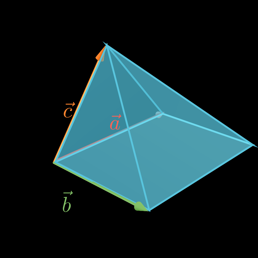
\end{align*} V = 3 1 ⋅ − 4 2 0 × − 4 − 3 5 ∘ − 2 0 10 = 3 1 ⋅ 10 20 20 ∘ − 2 0 10 = 3 1 ⋅ ∣ − 20 + 200∣ = 3 1 ⋅ 180 = 60 Volumen Pyramide mit dreieckiger Grundfläche 💡
Für das Volumen V V V a ⃗ , b ⃗ \vec a, \vec b a , b c ⃗ \vec c c
V = 1 6 ⋅ ∣ ( a ⃗ × b ⃗ ) ∘ c ⃗ ∣ V = \frac16\cdot
|(\vec a \times \vec b)
\circ \vec c \, | V = 6 1 ⋅ ∣ ( a × b ) ∘ c ∣ Beispiel a ⃗ = ( − 4 2 0 ) b ⃗ = ( − 4 − 3 5 ) c ⃗ = ( − 2 0 10 ) \vec a =
\left(\begin{matrix}
-4 \\ 2 \\ 0
\end{matrix}\right)
\qquad
\vec b =
\left(\begin{matrix}
-4 \\ -3 \\ 5
\end{matrix}\right)
\qquad
\vec c =
\left(\begin{matrix}
-2 \\ 0 \\ 10
\end{matrix}\right) a = − 4 2 0 b = − 4 − 3 5 c = − 2 0 10 V = 1 6 ⋅ ∣ [ ( − 4 2 0 ) × ( − 4 − 3 5 ) ] ∘ ( − 2 0 10 ) ∣ = 1 6 ⋅ ∣ ( 10 20 20 ) ∘ ( − 2 0 10 ) ∣ = 1 6 ⋅ ∣ − 20 + 200 ∣ = 1 6 ⋅ 180 = 30 \begin{align*}
V &= \frac16 \cdot
\left|
\left[
\left(\begin{matrix}
-4 \\ 2 \\ 0
\end{matrix}\right)
\times
\left(\begin{matrix}
-4 \\ -3 \\ 5
\end{matrix}\right)
\right]
\circ
\left(\begin{matrix}
-2 \\ 0 \\ 10
\end{matrix}\right)
\right|
\\
&= \frac16 \cdot
\left|
\left(\begin{matrix}
10 \\ 20 \\ 20
\end{matrix}\right)
\circ
\left(\begin{matrix}
-2 \\ 0 \\ 10
\end{matrix}\right)
\right|
\\&=\frac16 \cdot|{-20}+200|
\\&=\frac16 \cdot 180
\\&= 30
\end{align*} V = 6 1 ⋅ − 4 2 0 × − 4 − 3 5 ∘ − 2 0 10 = 6 1 ⋅ 10 20 20 ∘ − 2 0 10 = 6 1 ⋅ ∣ − 20 + 200∣ = 6 1 ⋅ 180 = 30 Spiegelung
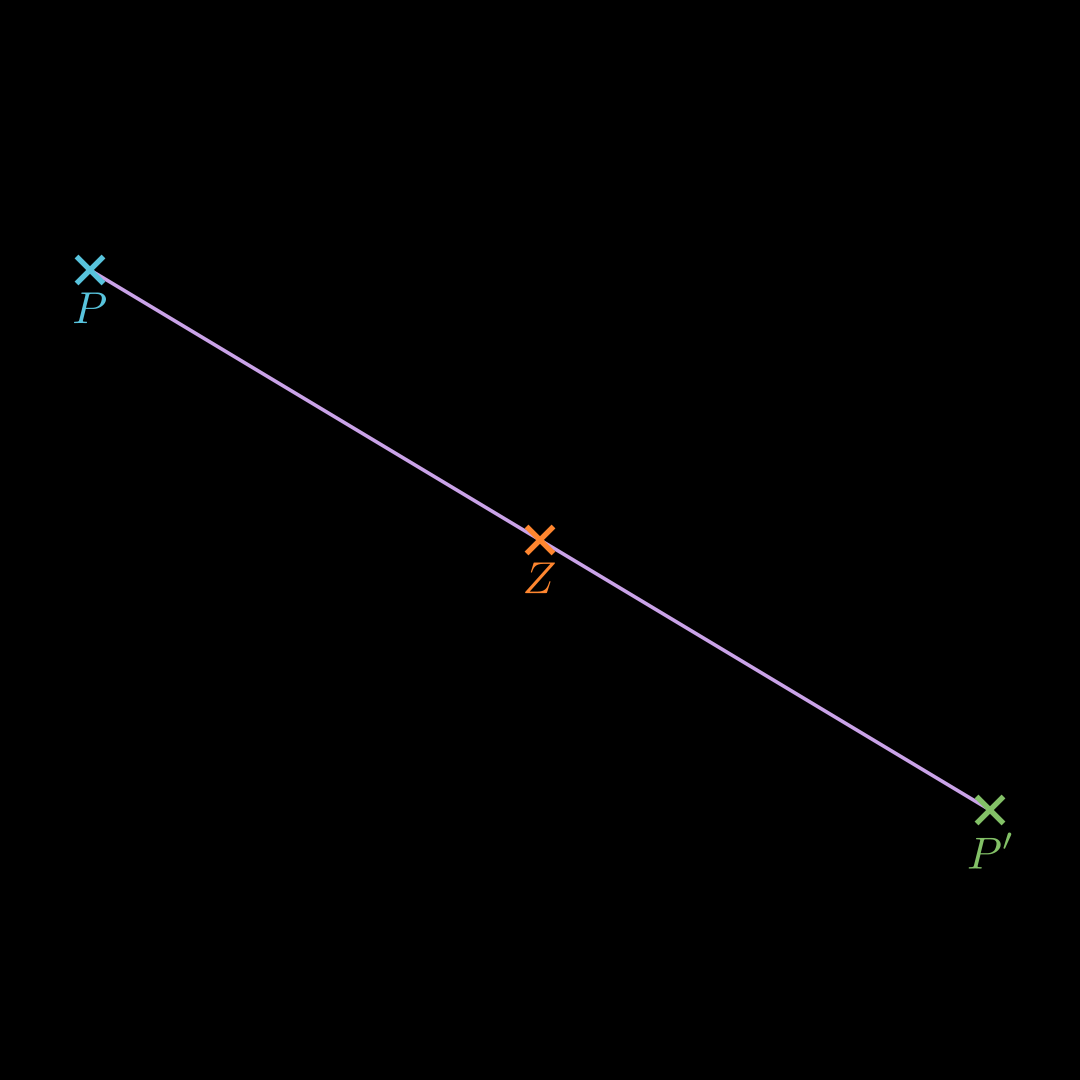
An einem Punkt spiegeln 💡
O P ′ → = O P → + 2 ⋅ P Z → = O Z → + P Z → \begin{align*}
\overrightarrow{OP'} &=
\overrightarrow{OP} + 2 \cdot \overrightarrow{PZ}\\
&=
\overrightarrow{OZ} +
\overrightarrow{PZ}
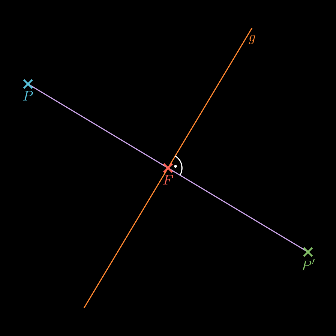
\end{align*} O P ′ = OP + 2 ⋅ PZ = OZ + PZ An einer Geraden spiegeln 💡
Stelle eine Hilfsebene H H H P P P g g g Erhalte den Punkt F F F g g g H H H Punktspiegelung an F F F O P ′ → = O F → + P F → \overrightarrow{OP'} = \overrightarrow{OF} + \overrightarrow{PF} O P ′ = OF + PF An einer Ebene Spiegeln 💡
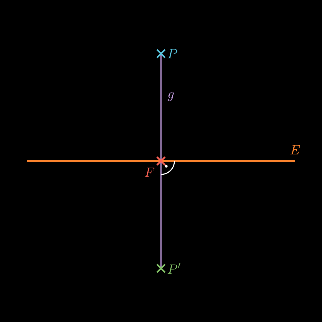
Stelle eine Gerade g g g E E E P P P Erhalte den Punkt F F F g g g E E E Punktspiegelung an F F F O P ′ → = O F → + P F → \overrightarrow{OP'} = \overrightarrow{OF} + \overrightarrow{PF} O P ′ = OF + PF Symmetrieebene bestimmen 💡
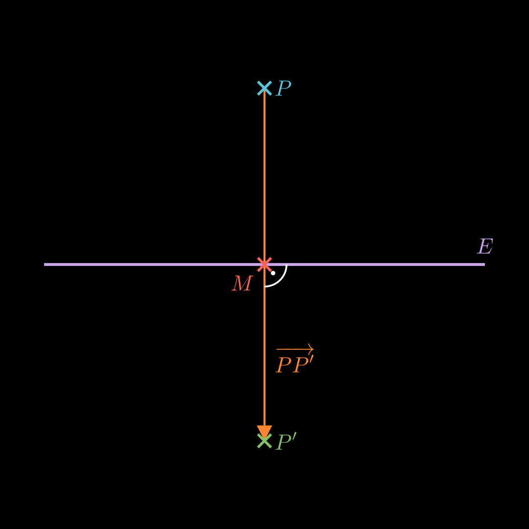
Berechne den Mittelpunkt M M M P P P P ’ P’ P ’ Stelle eine Gleichung für E E E M M M E E E P P ′ → \overrightarrow{PP'} P P ′ E E E
🔎