🔎
Ganzrationale Funktionen 💡
Eine ganzrationale Funktion f f f n n n
f ( x ) = a n x n + a n − 1 x n − 1 + . . . + a 1 x + a 0 f(x) = a_n x^n + a_{n-1} x^{n-1} + ... + a_1 x + a_0 f ( x ) = a n x n + a n − 1 x n − 1 + ... + a 1 x + a 0 mit a n ≠ 0 a_n \neq 0 a n = 0
Beispiele f ( x ) = x 2 − 4 x + 3 g ( x ) = 4 x 3 − 3 x 2 + x + 1 h ( x ) = 6 x 9 − 4 x 2 i ( x ) = 5 j ( x ) = 8 x 4 − 2 x 2 \begin{align*}
f(x) &= x^2 - 4x + 3 \\
g(x) &= 4x^3 - 3x^2 + x + 1 \\
h(x) &= 6x^9 - 4x^2 \\
i(x) &= 5 \\
j(x) &= 8x^4-2x^2
\end{align*} f ( x ) g ( x ) h ( x ) i ( x ) j ( x ) = x 2 − 4 x + 3 = 4 x 3 − 3 x 2 + x + 1 = 6 x 9 − 4 x 2 = 5 = 8 x 4 − 2 x 2 Nichtbeispiele f ( x ) = x g ( x ) = e x h ( x ) = sin ( x ) i ( x ) = x 2 x − 1 \begin{align*}
f(x) &= \sqrt x \\
g(x) &= e^x \\
h(x) &= \sin(x)\\
i(x) &= \frac{x^2}{x-1}
\end{align*} f ( x ) g ( x ) h ( x ) i ( x ) = x = e x = sin ( x ) = x − 1 x 2 Definitions- und Wertemenge 💡
Definitionsmenge Die Definitionsmenge D f D_f D f f f f x x x f ( x ) f(x) f ( x )
💡
Wertemenge Die Wertemenge W f W_f W f f f f f ( x ) f(x) f ( x )
Beispiele f ( x ) = x 2 D f = R W f = [ 0 ; ∞ [ \begin{align*}
f(x) &= x^2 \\
D_f &= \R \\
W_f &= [0; \infty[
\end{align*} f ( x ) D f W f = x 2 = R = [ 0 ; ∞ [ g ( x ) = ln ( x ) D g = ] 0 ; ∞ [ W g = R \begin{align*}
g(x) &= \ln(x) \\
D_g &= \ ]0; \infty[ \\
W_g &= \R
\end{align*} g ( x ) D g W g = ln ( x ) = ] 0 ; ∞ [ = R h ( x ) = 1 x D h = R ∖ { 0 } W h = R ∖ { 0 } \begin{align*}
h(x) &= \frac1x \\
D_h &= \R \setminus \{0\} \\
W_h &= \R \setminus \{0\}
\end{align*} h ( x ) D h W h = x 1 = R ∖ { 0 } = R ∖ { 0 } Potenzregel 💡
f ( x ) = a ⋅ x n ⇒ f ′ ( x ) = a ⋅ n ⋅ x n − 1 f(x) = a \cdot x^n
\quad\Rightarrow\quad
f'(x) = a \cdot n \cdot x^{n-1} f ( x ) = a ⋅ x n ⇒ f ′ ( x ) = a ⋅ n ⋅ x n − 1 Beispiele f ( x ) = x 2 f ′ ( x ) = 2 x \begin{align*}
f(x) &= x^2\\
f'(x) &= 2x
\end{align*} f ( x ) f ′ ( x ) = x 2 = 2 x g ( x ) = 1 x = x − 1 g ′ ( x ) = − 1 x 2 = − x − 2 \begin{align*}
g(x) &= \frac1x = x^{-1}\\
g'(x) &= -\frac1{x^2} = -x^-2
\end{align*} g ( x ) g ′ ( x ) = x 1 = x − 1 = − x 2 1 = − x − 2 h ( x ) = 3 x 2 h ′ ( x ) = 6 x \begin{align*}
h(x) &= 3x^2\\
h'(x) &= 6x
\end{align*} h ( x ) h ′ ( x ) = 3 x 2 = 6 x Verkettung von Funktionen 💡
u ∘ v = u ( v ( x ) ) u \circ v = u(v(x)) u ∘ v = u ( v ( x )) Die äußere Funktion u u u v v v
Beispiel u ( x ) = 1 − x 2 v ( x ) = 2 x + 1 ⇒ u ∘ v = 1 − ( 2 x + 1 ) 2 v ∘ u = 2 ( 1 − x 2 ) + 1 \begin{align*}
u(x) = 1 - x^2\\
v(x) = 2x + 1
\end{align*}
\quad\Rightarrow\quad
\begin{align*}
u \circ v = 1-(2x+1)^2\\
v \circ u = 2(1-x^2)+1
\end{align*} u ( x ) = 1 − x 2 v ( x ) = 2 x + 1 ⇒ u ∘ v = 1 − ( 2 x + 1 ) 2 v ∘ u = 2 ( 1 − x 2 ) + 1 Kettenregel 💡
f ( x ) = u ( v ( x ) ) ⇒ f ’ ( x ) = u ’ ( v ( x ) ) ⋅ v ’ ( x ) f(x) = u(v(x)) \quad\Rightarrow\quad f’(x) = u’(v(x)) \cdot v’(x) f ( x ) = u ( v ( x )) ⇒ f ’ ( x ) = u ’ ( v ( x )) ⋅ v ’ ( x ) Beispiel f ( x ) = ( 5 − 3 x ) 4 f ′ ( x ) = − 12 ( 5 − 3 x ) 3 u ( x ) = x 4 u ′ ( x ) = 4 x 3 v ( x ) = 5 − 3 x v ′ ( x ) = − 3 \begin{align*}
f(x) &= (5-3x)^4\\
f'(x) &= -12(5-3x)^3
\end{align*}
\quad
\begin{align*}
u(x) &= x^4\\
u'(x) &= 4x^3
\end{align*}
\quad
\begin{align*}
v(x) &= 5-3x\\
v'(x) &= -3
\end{align*} f ( x ) f ′ ( x ) = ( 5 − 3 x ) 4 = − 12 ( 5 − 3 x ) 3 u ( x ) u ′ ( x ) = x 4 = 4 x 3 v ( x ) v ′ ( x ) = 5 − 3 x = − 3 Produktregel 💡
f = u ⋅ v ⇒ f ’ = u ′ ⋅ v + u ⋅ v ′ f = u \cdot v \quad\Rightarrow\quad
f’ = u' \cdot v + u \cdot v' f = u ⋅ v ⇒ f ’ = u ′ ⋅ v + u ⋅ v ′ Beispiel f ( x ) = 2 x ⋅ x 2 + 1 f ′ ( x ) = 2 x 2 + 1 + 2 x 2 x 2 + 1 u ( x ) = 2 x u ′ ( x ) = 2 v ( x ) = x 2 + 1 v ′ ( x ) = x x 2 + 1 \begin{align*}
f(x) &= 2x \cdot \sqrt{x^2+1}\\
f'(x) &= 2\sqrt{x^2+1}+\frac{2x^2}{\sqrt{x^2+1}}
\end{align*}
\qquad
\begin{align*}
u(x) &= 2x\\
u'(x) &= 2
\end{align*}
\qquad
\begin{align*}
v(x) &= \sqrt{x^2+1}\\
v'(x) &= \frac{x}{\sqrt{x^2+1}}
\end{align*} f ( x ) f ′ ( x ) = 2 x ⋅ x 2 + 1 = 2 x 2 + 1 + x 2 + 1 2 x 2 u ( x ) u ′ ( x ) = 2 x = 2 v ( x ) v ′ ( x ) = x 2 + 1 = x 2 + 1 x Quotientenregel 💬
Die Quotientenregel ist kein offizieller Abiturstoff.
💡
f = u v ⇒ f ’ = u ′ ⋅ v − u ⋅ v ′ v 2 f = \frac uv \quad\Rightarrow\quad
f’ = \frac{u' \cdot v - u \cdot v'}{v^2} f = v u ⇒ f ’ = v 2 u ′ ⋅ v − u ⋅ v ′ Beispiel f ( x ) = x 2 x 2 − 3 f ′ ( x ) = 2 x ⋅ ( x 2 − 3 ) − x 2 ⋅ 2 x ( x 2 − 3 ) 2 u ( x ) = x 2 u ′ ( x ) = 2 x v ( x ) = x 2 − 3 v ′ ( x ) = 2 x \begin{align*}
f(x) &= \frac{x^2}{x^2-3}\\
f'(x) &= \frac{2x\cdot(x^2-3)-x^2\cdot2x}{(x^2-3)^2}
\end{align*}
\qquad
\begin{align*}
u(x) &= x^2\\
u'(x) &= 2x
\end{align*}
\qquad
\begin{align*}
v(x) &= x^2-3\\
v'(x) &= 2x
\end{align*} f ( x ) f ′ ( x ) = x 2 − 3 x 2 = ( x 2 − 3 ) 2 2 x ⋅ ( x 2 − 3 ) − x 2 ⋅ 2 x u ( x ) u ′ ( x ) = x 2 = 2 x v ( x ) v ′ ( x ) = x 2 − 3 = 2 x Monotonie Definition 💡
Gegeben ist eine Funktion f f f I I I
f f f streng monoton wachsend auf I I I x 1 , x 2 ∈ I x_1, x_2 \in I x 1 , x 2 ∈ I
x 1 < x 2 ⇒ f ( x 1 ) < f ( x 2 ) x_1 < x_2 \quad\Rightarrow\quad f(x_1) < f(x_2) x 1 < x 2 ⇒ f ( x 1 ) < f ( x 2 ) f f f streng monoton fallend auf I I I wenn für alle x 1 , x 2 ∈ I x_1, x_2 \in I x 1 , x 2 ∈ I
x 1 < x 2 ⇒ f ( x 1 ) > f ( x 2 ) x_1 < x_2 \quad\Rightarrow\quad f(x_1) > f(x_2) x 1 < x 2 ⇒ f ( x 1 ) > f ( x 2 ) Gilt „nur“ f ( x 1 ) ≤ f ( x 2 ) f(x_1)\leq f(x_2) f ( x 1 ) ≤ f ( x 2 ) f ( x 1 ) ≥ f ( x 2 ) f(x_1) ≥ f(x_2) f ( x 1 ) ≥ f ( x 2 ) f f f monoton wachsend bzw. fallend .
Satz 💡
Ist die Funktion f f f I I I
a) f ′ ( x ) > 0 f'(x) > 0 f ′ ( x ) > 0 x ∈ I ⇒ f x \in I\quad\Rightarrow\quad f x ∈ I ⇒ f streng monoton wachsend auf I I I
b) f ′ ( x ) < 0 f'(x) < 0 f ′ ( x ) < 0 x ∈ I ⇒ f x \in I\quad\Rightarrow\quad f x ∈ I ⇒ f streng monoton fallend auf I I I
⚠️
Der Monotoniesatz kann irreführende Ergebnisse liefern. Zum Beispiel ist f ( x ) = x 3 f(x) = x^3 f ( x ) = x 3 f ′ ( 0 ) = 0 f'(0) = 0 f ′ ( 0 ) = 0
Krümmung Definition 💡
Ist die Funktion f f f
a) …steigend, so beschreibt der Graph von f f f
b) …fallend, so beschreibt der Graph von f f f
Satz 💡
Ist die Funktion f f f I I I
a) f ′ ′ ( x ) > 0 f''(x) > 0 f ′′ ( x ) > 0 x ∈ I ⇒ x \in I\quad\Rightarrow\quad x ∈ I ⇒ f f f
b) f ′ ′ ( x ) < 0 f''(x) < 0 f ′′ ( x ) < 0 x ∈ I ⇒ x \in I\quad\Rightarrow\quad x ∈ I ⇒ f f f
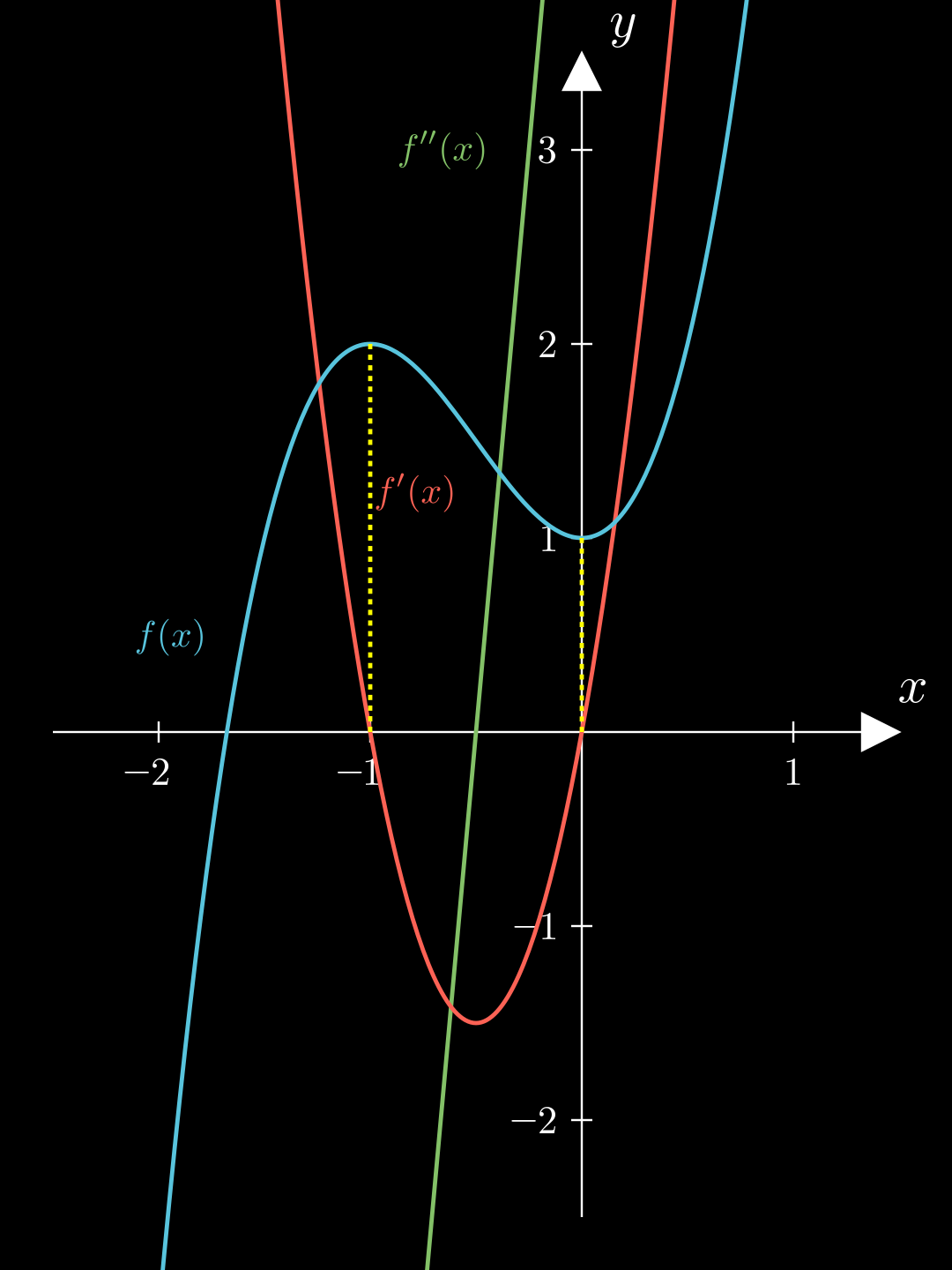
Beispiel f ′ ′ ( − 0 , 5 ) = 0 f ′ ′ ( − 1 ) < 0 f ′ ′ ( 0 ) > 0 \begin{align*}
f''(-0{,}5) &= 0 \\
f''(-1) &< 0 \\
f''(0) &> 0
\end{align*} f ′′ ( − 0 , 5 ) f ′′ ( − 1 ) f ′′ ( 0 ) = 0 < 0 > 0 f ′ ′ f'' f ′′ x = − 0 , 5 x = -0,5 x = − 0 , 5 f ′ ′ < 0 f'' < 0 f ′′ < 0 f ′ ′ > 0 f''>0 f ′′ > 0 f f f 0 , 5 0{,}5 0 , 5 0 , 5 0{,}5 0 , 5
Extremstellen 💡
Ist f f f I I I innere Extremstelle x 0 ∈ I x_0 \in I x 0 ∈ I f f f
notwendige Bedingung: f ′ ( x 0 ) = 0 f'(x_0) = 0 f ′ ( x 0 ) = 0 hinreichende Bedingung: x 0 x_0 x 0 ist ein Maximum , wenn f ′ ( x ) f'(x) f ′ ( x ) an x 0 x_0 x 0 sein Vorzeichen von + nach - wechselt, oder wenn f ′ ′ ( x 0 ) < 0 f''(x_0)<0 f ′′ ( x 0 ) < 0 ist.
x 0 x_0 x 0 ist ein Minimum , wenn f ′ ( x ) f'(x) f ′ ( x ) an x 0 x_0 x 0 sein Vorzeichen von - nach + wechselt, oder wenn f ′ ′ ( x 0 ) > 0 f''(x_0) > 0 f ′′ ( x 0 ) > 0 ist.
⚠️
Ist f ′ ′ ( x 0 ) = 0 f''(x_0) = 0 f ′′ ( x 0 ) = 0 f ′ f' f ′
Nur wenn die notwendige und die hinreichende Bedingung erfüllt sind, ist x 0 x_0 x 0
Beispiele f ′ ( − 1 ) = 0 ⇒ f ′ ( 0 ) = 0 ⇒ f ′ ′ ( − 1 ) < 0 ⇒ f ′ ′ ( 0 ) > 0 ⇒ Maximum Minimum \begin{align*}
f'(-1) &= 0 \quad\Rightarrow\quad\\
f'(0) &= 0 \quad\Rightarrow\quad
\end{align*}
\begin{align*}
f''(-1) &< 0 \quad\Rightarrow\quad\\
f''(0) &> 0 \quad\Rightarrow\quad
\end{align*}
\begin{align*}
&\textsf{Maximum}\\
&\textsf{Minimum}
\end{align*} f ′ ( − 1 ) f ′ ( 0 ) = 0 ⇒ = 0 ⇒ f ′′ ( − 1 ) f ′′ ( 0 ) < 0 ⇒ > 0 ⇒ Maximum Minimum g ( x ) = x 4 g ′ ( x ) = 4 x 3 g ′ ′ ( x ) = 12 x 2 g ′ ( x ) = 0 ⇒ x = 0 g ′ ′ ( 0 ) = 0 Vorzeichen u ¨ berpr u ¨ fen: g ′ ( − 1 ) = − 4 g ′ ( 1 ) = 4 ⇒ - zu +: Minimum g(x) = x^4 \quad
g'(x) = 4x^3 \quad
g''(x) = 12x^2\\
\begin{align*}
\\g'(x) &= 0 \ \ \Rightarrow \ \
x = 0\\
g''(0) &= 0 \\\\
\textsf{Vorzeichen }& \textsf{überprüfen:} \\
g'(-1) &= -4 \\
g'(1) &= 4 \\
\Rightarrow
\textsf{- zu +: }&\textsf{Minimum}
\end{align*} g ( x ) = x 4 g ′ ( x ) = 4 x 3 g ′′ ( x ) = 12 x 2 g ′ ( x ) g ′′ ( 0 ) Vorzeichen g ′ ( − 1 ) g ′ ( 1 ) ⇒ - zu +: = 0 ⇒ x = 0 = 0 u ¨ berpr u ¨ fen: = − 4 = 4 Minimum Wendestellen 💡
Ist f f f I I I x 0 ∈ I x_0 \in I x 0 ∈ I Wendestelle von f f f
f ′ ′ ( x 0 ) = 0 f''(x_0) = 0 f ′′ ( x 0 ) = 0 f ′ ′ ( x ) f''(x) f ′′ ( x ) x 0 x_0 x 0
oder f ′ ′ ( x 0 ) = 0 und f ′ ′ ′ ( x 0 ) ≠ 0 \textsf{oder}\\ {}\\
f''(x_0)=0
\quad\textsf{und}\quad
f'''(x_0) \neq 0 oder f ′′ ( x 0 ) = 0 und f ′′′ ( x 0 ) = 0 ⚠️
Ähnlich wie bei den Extremstellen muss man den Vorzeichenwechsel nur überprüfen, wenn f ′ ′ ′ ( x 0 ) = 0 f'''(x_0) = 0 f ′′′ ( x 0 ) = 0
Beispiel f ′ ′ ′ f''' f ′′′
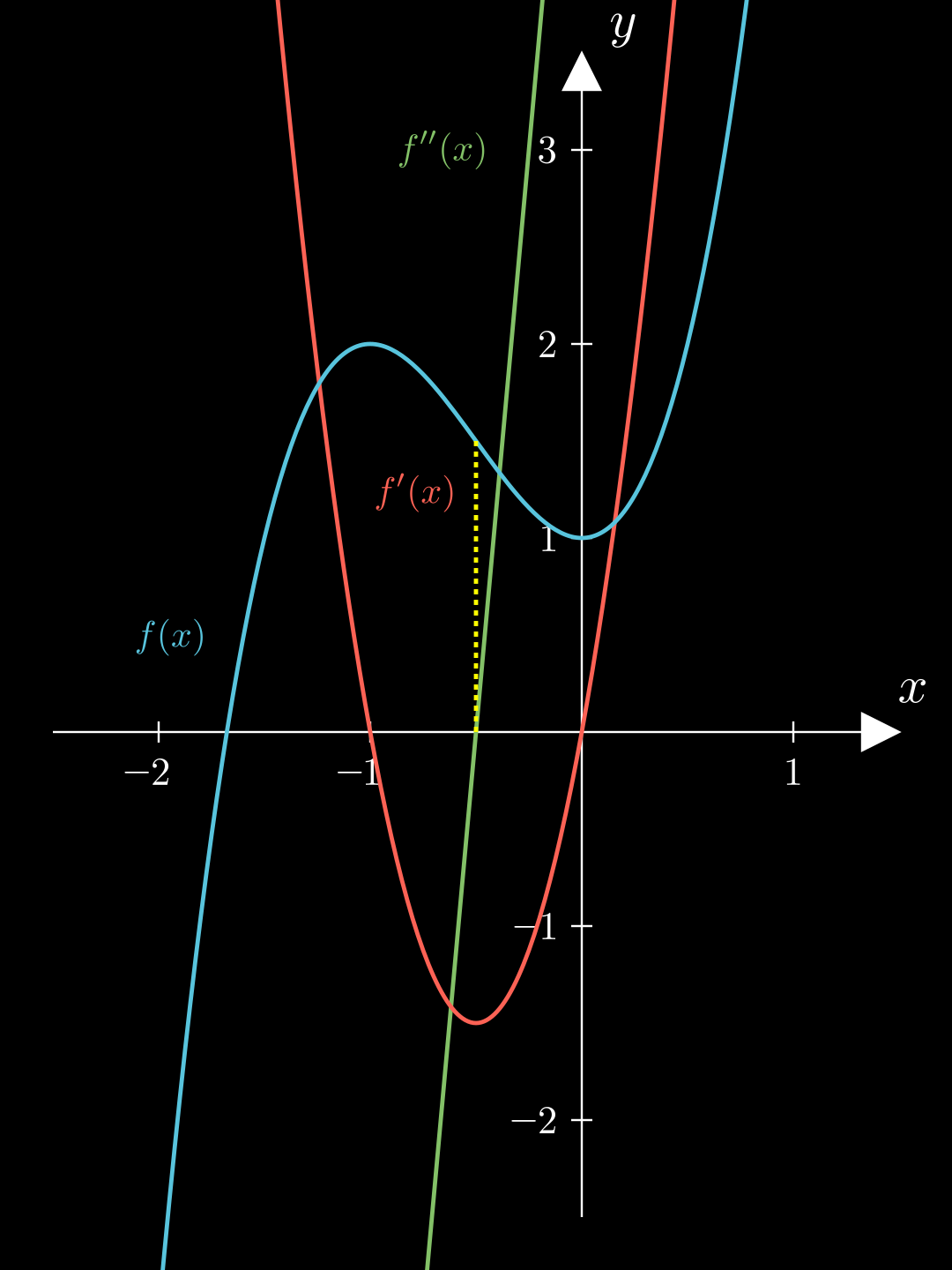
f ′ ′ ( − 0 , 5 ) = 0 f ′ ′ ′ ( − 0 , 5 ) ≠ 0 ⇒ Wendestelle bei x = 0 , 5 \begin{align*}
f''(-0{,}5) &= 0 \\
f'''(-0{,}5) &\neq 0 \\
\Rightarrow
\textsf{Wendestelle } & \textsf{bei } x = 0{,}5
\end{align*} f ′′ ( − 0 , 5 ) f ′′′ ( − 0 , 5 ) ⇒ Wendestelle = 0 = 0 bei x = 0 , 5 h ( x ) = x 4 h ′ ( x ) = 4 x 3 h ′ ′ ( x ) = 12 x 2 h ′ ′ ′ ( x ) = 24 x h ′ ′ ( x ) = 0 ⇒ x = 0 h ′ ′ ′ ( 0 ) = 0 Vorzeichen u ¨ berpr u ¨ fen: h ′ ′ ( − 1 ) = 12 h ′ ′ ( 1 ) = 12 ⇒ + zu +: kein Wendepunkt h(x) = x^4 \qquad
h'(x) = 4x^3 \\
h''(x) = 12x^2 \quad
h'''(x) = 24x\\
\begin{align*}
\\h''(x) &= 0 \ \ \Rightarrow \ \
x = 0\\
h'''(0) &= 0 \\\\
\textsf{Vorzeichen }& \textsf{überprüfen:} \\
h''(-1) &= 12 \\
h''(1) &= 12 \\
\Rightarrow
\textsf{+ zu +: }&
\textsf{kein Wendepunkt}
\end{align*} h ( x ) = x 4 h ′ ( x ) = 4 x 3 h ′′ ( x ) = 12 x 2 h ′′′ ( x ) = 24 x h ′′ ( x ) h ′′′ ( 0 ) Vorzeichen h ′′ ( − 1 ) h ′′ ( 1 ) ⇒ + zu +: = 0 ⇒ x = 0 = 0 u ¨ berpr u ¨ fen: = 12 = 12 kein Wendepunkt Tangenten- und Normalengleichung Allgemeine Geradengleichung: y = m ⋅ x + c y = m\cdot x +c y = m ⋅ x + c
Tangentengleichung Für die Tangente t t t u u u f f f
💡
t : y = f ′ ( u ) ⋅ ( x − u ) + f ( u ) t: y = f'(u) \cdot (x-u) + f(u) t : y = f ′ ( u ) ⋅ ( x − u ) + f ( u ) Normalengleichung Für die Normale n n n u u u f f f
💡
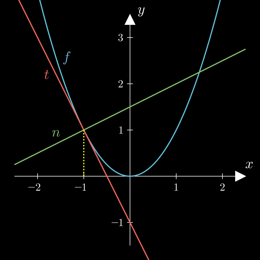
n : y = − 1 f ′ ( u ) ⋅ ( x − u ) + f ( u ) n: y = -\frac{1}{f'(u)} \cdot (x-u) + f(u) n : y = − f ′ ( u ) 1 ⋅ ( x − u ) + f ( u ) Erklärung Beispiel f ( x ) = x 2 f ′ ( x ) = 2 x u = − 1 f ( u ) = f ( − 1 ) = 1 f ′ ( u ) = f ′ ( − 1 ) = − 2 f(x) = x^2 \quad f'(x) = 2x \\
u=-1
\\{}\\
\begin{align*}
f(u)&=f(-1) = 1\\
f'(u)&=f'(-1) = -2\\
\end{align*} f ( x ) = x 2 f ′ ( x ) = 2 x u = − 1 f ( u ) f ′ ( u ) = f ( − 1 ) = 1 = f ′ ( − 1 ) = − 2 t : y = − 2 ( x − ( − 1 ) ) + 1 = − 2 x − 1 n : y = − 1 − 2 ( x + 1 ) + 1 = 1 2 x + 3 2 \begin{align*}
t: y &= -2(x-(-1))+1\\
&=-2x-1\\ \\
n: y&= -\frac1{-2}
(x+1)+1\\
&=\frac12x+\frac32
\end{align*} t : y n : y = − 2 ( x − ( − 1 )) + 1 = − 2 x − 1 = − − 2 1 ( x + 1 ) + 1 = 2 1 x + 2 3 Differentialquotient 💡
Eine Funktion f ′ f' f ′ a a a f ( a + h ) − f ( a ) h \frac{f(a+h)-f(a)}{h} h f ( a + h ) − f ( a ) h → 0 h \to 0 h → 0 f f f a a a
f ′ ( a ) = lim h → 0 f ( a + h ) − f ( a ) h f'(a) = \lim_{h \to 0} \frac{f(a+h)-f(a)}{h} f ′ ( a ) = h → 0 lim h f ( a + h ) − f ( a ) nicht alle Funktionen sind (überall) differenzierbar f ( x ) = x f ( 0 ) = 0 ⇒ f ′ ( x ) = 1 2 x f ′ ( 0 ) = 1 0 ⇒ × \begin{align*}
f(x) &= \sqrt x \\
f(0) &= 0\
\end{align*}
\quad\Rightarrow\quad
\begin{align*}
f'(x) &= \frac1{2\sqrt x}\\
f'(0) &= \frac10 \Rightarrow\times
\end{align*} f ( x ) f ( 0 ) = x = 0 ⇒ f ′ ( x ) f ′ ( 0 ) = 2 x 1 = 0 1 ⇒ × Die Wurzelfunktion ist für x = 0 x=0 x = 0
Beispiel f ( x ) = x 2 f ′ ( a ) = lim h → 0 ( a + h ) 2 − a 2 h f ′ ( a ) = lim h → 0 a 2 + 2 a h + h 2 − a 2 h f ′ ( a ) = lim h → 0 2 a + h f ′ ( a ) = 2 a \begin{align*}
f(x) &= x^2\\
f'(a) &= \lim_{h \to 0} \frac{(a+h)^2 - a^2}{h}\\
f'(a) &= \lim_{h \to 0} \frac{a^2 + 2ah + h^2 - a^2}{h}\\
f'(a) &= \lim_{h \to 0} 2a+h\\
f'(a) &=2a
\end{align*} f ( x ) f ′ ( a ) f ′ ( a ) f ′ ( a ) f ′ ( a ) = x 2 = h → 0 lim h ( a + h ) 2 − a 2 = h → 0 lim h a 2 + 2 ah + h 2 − a 2 = h → 0 lim 2 a + h = 2 a 💬
Dass man das im Abi machen muss, ist sehr unwahrscheinlich, aber grob zu wissen, wie es geht, kann nicht schaden.
Berührpunkte von Funktionsgraphen 💡
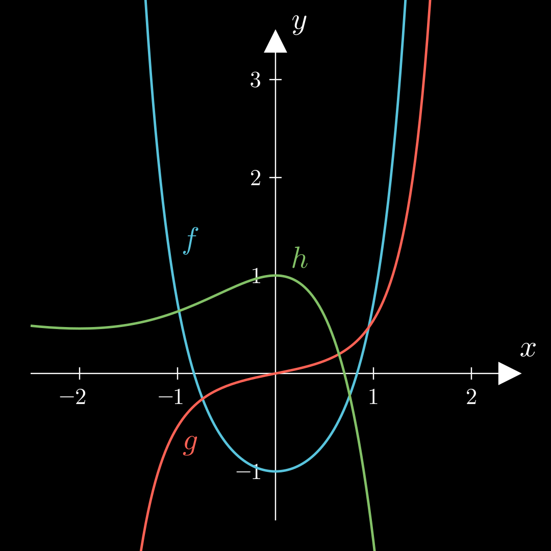
Die Graphen der Funktionen von f f f g g g u u u
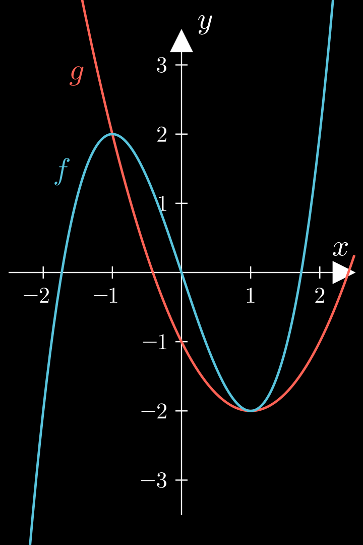
f ( u ) = g ( u ) und f ′ ( u ) = g ′ ( u ) f(u) = g(u) \quad \textsf{und} \quad f'(u) = g'(u) f ( u ) = g ( u ) und f ′ ( u ) = g ′ ( u ) Beispiel f ( x ) = x 3 − 3 x f ′ ( x ) = 3 x 2 − 3 g ( x ) = x 2 − 2 x − 1 g ′ ( x ) = 2 x − 2 \begin{align*}
f(x) &= x^3-3x \\
f'(x) &= 3x^2-3
\end{align*}
\qquad
\begin{align*}
g(x) &= x^2 - 2x -1 \\
g'(x) &= 2x - 2
\end{align*} f ( x ) f ′ ( x ) = x 3 − 3 x = 3 x 2 − 3 g ( x ) g ′ ( x ) = x 2 − 2 x − 1 = 2 x − 2 f ( x ) = g ( x ) ⇒ x 1 = 1 x 2 = − 1 f(x) = g(x) \\
\Rightarrow x_1 = 1 \quad x_2 = -1
f ( x ) = g ( x ) ⇒ x 1 = 1 x 2 = − 1 x 1 : f ( 1 ) = − 2 = g ( 1 ) = − 2 ✓ f ′ ( 1 ) = 0 = g ′ ( 1 ) = 0 ✓ ⇒ Die Graphen von f und g ber u ¨ hren sich bei x = 1 x_1: \\
f(1) = -2 = g(1) = -2
\ \checkmark \\
f'(1) = 0 = g'(1) = 0
\ \checkmark \\
\Rightarrow \textsf{Die Graphen von } f \textsf{ und } g \textsf{ berühren sich bei } x = 1 x 1 : f ( 1 ) = − 2 = g ( 1 ) = − 2 ✓ f ′ ( 1 ) = 0 = g ′ ( 1 ) = 0 ✓ ⇒ Die Graphen von f und g ber u ¨ hren sich bei x = 1 x 2 : f ( − 1 ) = 2 = g ( − 1 ) = 2 ✓ f ′ ( − 1 ) = 0 = g ′ ( − 1 ) = − 4 × ⇒ Die Graphen von f und g schneiden sich bei x = − 1 x_2: \\
f(-1) = 2 = g(-1) = 2
\ \checkmark \\
f'(-1) = 0 = g'(-1) = -4
\ \times \\
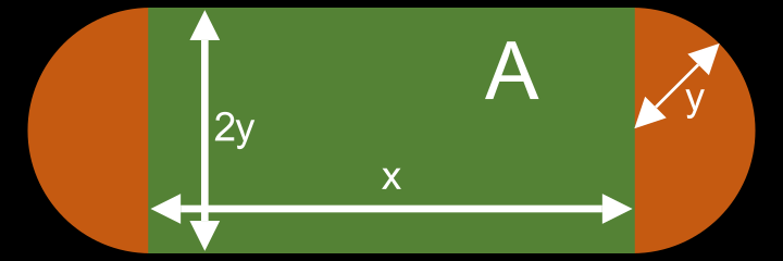
\Rightarrow \textsf{Die Graphen von } f \textsf{ und } g \textsf{ schneiden sich bei } x = -1 x 2 : f ( − 1 ) = 2 = g ( − 1 ) = 2 ✓ f ′ ( − 1 ) = 0 = g ′ ( − 1 ) = − 4 × ⇒ Die Graphen von f und g schneiden sich bei x = − 1 Extremwertprobleme Beispiel Eine Sportstadion mit einer Laufbahn von 400m Länge soll so angelegt werden, dass die Fläche A A A
Aufstellen eines Terms der möglichst groß/klein werden soll Fl a ¨ che Fußballfeld: A = x ⋅ 2 y \text{Fläche Fußballfeld: } \\
A = x \cdot2y Fl a ¨ che Fußballfeld: A = x ⋅ 2 y Formulieren von NebenbedingungenL a ¨ nge Laufbahn: 2 x + 2 y π = 400 ∣ − 2 x ∣ : 2 π y = 200 − x π \text{Länge Laufbahn: } \\
\begin{align*}
2x+2y\pi &= 400
\quad |-2x \quad |:2\pi
\\
y &= \frac{200-x}\pi
\end{align*} L a ¨ nge Laufbahn: 2 x + 2 y π y = 400 ∣ − 2 x ∣ : 2 π = π 200 − x Aufstellen der Zielfunktion und Angeben ihrer Definitionsmenge A ( x ) = x ⋅ 2 ( 200 − x π ) = 400 x − 2 x 2 π = − 2 π x 2 + 400 π x D A = [ 0 ; 200 ] \begin{align*}
A(x) &= x\cdot2(\frac{200-x}{\pi})
= \frac{400x-2x^2}{\pi}
= \frac{-2}{\pi}x^2+ \frac{400}{\pi}x
\\
D_A &= [0; 200]
\end{align*} A ( x ) D A = x ⋅ 2 ( π 200 − x ) = π 400 x − 2 x 2 = π − 2 x 2 + π 400 x = [ 0 ; 200 ] Untersuchen der Zielfunktion nach Maxima/Minima unter Beachtung von Randextrema A ( 0 ) = A ( 200 ) = 0 A ′ ( x ) = − 4 π x + 400 π A ′ ( x ) = 0 0 = − 4 π x + 400 π ∣ ⋅ π 4 0 = − x + 100 ∣ + x x = 100 ⇒ y ≈ 31 , 8 m A ≈ 6366 m 2 \begin{align*}
A(0) &= A(200) = 0 \\ \\
A'(x) &= \frac{-4}{\pi}x + \frac{400}{\pi} \\
A'(x) &= 0 \\
0 &= \frac{-4}{\pi}x + \frac{400}{\pi}
\quad |\cdot \frac{\pi}4
\\
0 &= -x + 100 \qquad |+x \\
x &= 100
\end{align*}
\\
\Rightarrow
y \approx 31{,8}m \quad
A \approx 6366m^2 A ( 0 ) A ′ ( x ) A ′ ( x ) 0 0 x = A ( 200 ) = 0 = π − 4 x + π 400 = 0 = π − 4 x + π 400 ∣ ⋅ 4 π = − x + 100 ∣ + x = 100 ⇒ y ≈ 31 , 8 m A ≈ 6366 m 2 Eulersche Zahl und natürlicher Logarithmus 💡
Die eulersche Zahl e ≈ 2 , 72 e \thickapprox 2{,}72 e ≈ 2 , 72
f ( x ) = e x f ′ ( x ) = e x f(x) = e^x \qquad f'(x) = e^x \\ f ( x ) = e x f ′ ( x ) = e x 💡
Der natürliche Logarithmus ln \ln ln e e e ln \ln ln
e x = a x = ln ( a ) und f ( x ) = ln ( x ) f ′ ( x ) = 1 x \begin{align*}
e^x &= a \\
x &= \ln(a)
\end{align*}
\qquad \textsf{und} \qquad
\begin{align*}
f(x) &= \ln(x) \\
f'(x) &= \frac1x
\end{align*} e x x = a = ln ( a ) und f ( x ) f ′ ( x ) = ln ( x ) = x 1
Rechenregeln Potenzen und Logarithmen 💡
x a ⋅ x b = x a + b x a x b = x a − b x a b = x a ⋅ b ln ( a ⋅ b ) = ln ( a ) + ln ( b ) ln ( a b ) = ln ( a ) − ln ( b ) ln ( a b ) = b ⋅ ln ( a ) \begin{align*}
x^a \cdot x^b &= x^{a+b} \\
\frac{x^a}{x^b} &= x^{a-b} \\
x^{a^b} &= x^{a \cdot b}
\end{align*}
\qquad\qquad
\begin{align*}
\ln(a \cdot b) &= \ln(a) + \ln(b) \\
\ln(\frac ab) &= \ln(a) - \ln(b) \\
\ln(a^b) &= b \cdot \ln(a)
\end{align*} x a ⋅ x b x b x a x a b = x a + b = x a − b = x a ⋅ b ln ( a ⋅ b ) ln ( b a ) ln ( a b ) = ln ( a ) + ln ( b ) = ln ( a ) − ln ( b ) = b ⋅ ln ( a ) Die Logarithmusgesetze gelten für alle Logarithmusfunktionen, nicht nur für den natürlichen Logarithmus.
Beispiele ln ( 1 e ) = ln ( 1 ) − ln ( e ) = − 1 ln ( e 4 ⋅ e 2 ) = ln ( e 4 ) + ln ( e 2 ) = 6 = ln ( e 6 ) = 6 \begin{align*}
\ln(\frac1e) &= \ln(1)-\ln(e) = -1
\\ \\
\ln(e^4 \cdot e^2)
&= \ln(e^4) + \ln(e^2) = 6\\
&= \ln(e^6) = 6
\end{align*} ln ( e 1 ) ln ( e 4 ⋅ e 2 ) = ln ( 1 ) − ln ( e ) = − 1 = ln ( e 4 ) + ln ( e 2 ) = 6 = ln ( e 6 ) = 6 8 16 8 6 = 8 6 e − 2 ⋅ ln ( 4 ) = ( e ln ( 4 ) ) − 2 = 4 − 2 = 1 16 = e ln ( 4 − 2 ) = 4 − 2 = 1 16 \begin{align*}
\frac{8^{16}}{8^{6}} &= 8^6
\\ \\
e^{-2 \cdot \ln(4)}
&= (e^{\ln(4)})^{-2} &= 4^{-2} &= \frac1{16} \\
&= e^{\ln(4^{-2})} &= 4^{-2} &= \frac1{16}
\end{align*} 8 6 8 16 e − 2 ⋅ l n ( 4 ) = 8 6 = ( e l n ( 4 ) ) − 2 = e l n ( 4 − 2 ) = 4 − 2 = 4 − 2 = 16 1 = 16 1 Verhalten von Exponentialfunktionen im Unendlichen 💡
Bei Funktionen der Form f ( x ) = x n ⋅ e a ⋅ x ( a ≠ 0 ) f(x) = x^n \cdot e^{a\cdot x} \ (a \neq 0) f ( x ) = x n ⋅ e a ⋅ x ( a = 0 ) e a ⋅ x e^{a \cdot x} e a ⋅ x x → ± ∞ x \rightarrow \pm \infty x → ± ∞ x n x^n x n
Beispiele → 0 \rightarrow 0 → 0 → 0 \rightarrow 0 → 0 → + ∞ \rightarrow +\infty → + ∞ → + ∞ \rightarrow +\infty → + ∞ → − ∞ \rightarrow -\infty → − ∞ → + ∞ \rightarrow +\infty → + ∞ → 0 \rightarrow 0 → 0 → + ∞ \rightarrow +\infty → + ∞
Symmetrie von Funktionsgraphen 💡
Der Graph von f f f achsensymmetrisch zur y-Achse , wenn für alle x ∈ D f : f ( − x ) = f ( x ) x \in D_f : f(-x) = f(x) x ∈ D f : f ( − x ) = f ( x )
Der Graph von f f f punksymmetrisch um Ursprung , wenn für alle x ∈ D f : f ( − x ) = − f ( x ) x \in D_f : f(-x) = -f(x) x ∈ D f : f ( − x ) = − f ( x )
Beispiele f ( x ) = e x 2 + 4 f ( − x ) = e ( − x ) 2 + 4 = e x 2 + 4 = f ( x ) ⇒ Der Graph von f ist achsensymmetrisch zur y-Achse \begin{align*}
f(x) &= e^{x^2} + 4 \\
f(-x) &= e^{(-x)^2} + 4 \\
&= e^{x^2}+4 \\
&= f(x) \\
\Rightarrow
\textsf{Der Graph von } &f
\textsf{ ist achsensymmetrisch zur y-Achse}
\end{align*} f ( x ) f ( − x ) ⇒ Der Graph von = e x 2 + 4 = e ( − x ) 2 + 4 = e x 2 + 4 = f ( x ) f ist achsensymmetrisch zur y-Achse g ( x ) = 1 5 x ⋅ e x 2 g ( − x ) = 1 5 ( − x ) ⋅ e ( − x ) 2 = − 1 5 x ⋅ e x 2 = − g ( x ) ⇒ Der Graph von f ist punktsymmetrisch zum Ursprung \begin{align*}
g(x) &=
\frac15 x \cdot e^{x^2} \\
g(-x) &=
\frac15 (-x) \cdot e^{(-x)^2} \\
&= -\frac15 x \cdot e^{x^2} \\
&= -g(x) \\
\Rightarrow
\textsf{Der Graph von } &f
\textsf{ ist punktsymmetrisch zum Ursprung}
\end{align*} g ( x ) g ( − x ) ⇒ Der Graph von = 5 1 x ⋅ e x 2 = 5 1 ( − x ) ⋅ e ( − x ) 2 = − 5 1 x ⋅ e x 2 = − g ( x ) f ist punktsymmetrisch zum Ursprung
h ( x ) = − x 2 ⋅ e x + 1 h ( − x ) = − ( − x ) 2 ⋅ e − x + 1 = − x 2 ⋅ e − x + 1 ⇒ keine Sy mmetrie erkennbar ‾ \begin{align*}
h(x) &= -x^2 \cdot e^x + 1 \\
h(-x) &= -(-x)^2 \cdot e^{-x} + 1 \\
&= -x^2 \cdot e^{-x} + 1\\
\Rightarrow
\textsf{keine Sy}
&\textsf{mmetrie \underline{erkennbar}}
\end{align*} h ( x ) h ( − x ) ⇒ keine Sy = − x 2 ⋅ e x + 1 = − ( − x ) 2 ⋅ e − x + 1 = − x 2 ⋅ e − x + 1 mmetrie erkennbar ⚠️
Diese Methode funktioniert nur, um die Symmetrie zur y-Achse oder zum Ursprung zu bestimmen.
f ( x ) = ( x − 2 ) 2 f(x) = (x-2)^2 f ( x ) = ( x − 2 ) 2 x = 2 x=2 x = 2 f f f
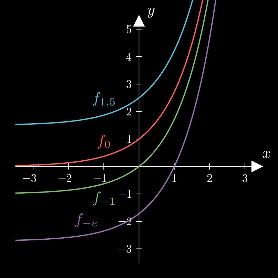
Funktionsschar 💡
Enthält eine Funktion f f f x x x Parameter k k k k k k f k f_k f k f k f_k f k Funktionsschar .
Beispiel f k ( x ) = e x + k f k ′ ( x ) = e x f 0 ( x ) = e x f 1 ( x ) = e x + 1 usw. \begin{align*}
f_k(x) = e^x + k \qquad
f'_k(x) = e^x \\
\\
f_0(x) = e^x \qquad f_1(x) = e^x + 1 \quad\textsf{usw.}
\end{align*} f k ( x ) = e x + k f k ′ ( x ) = e x f 0 ( x ) = e x f 1 ( x ) = e x + 1 usw. Nullstellen in Abhängigkeit von k k k :
f k ( x ) = 0 0 = e x + k ∣ − k − k = e x ∣ ln , k < 0 x = ln ( − k ) , k < 0 \begin{align*}
f_k(x) &= 0 \\
0 &= e^x + k \quad|-k \\
-k &= e^x \qquad \ \ \ |\ln, k < 0 \\
x &= \ln(-k), \quad k < 0
\end{align*} f k ( x ) 0 − k x = 0 = e x + k ∣ − k = e x ∣ ln , k < 0 = ln ( − k ) , k < 0
Umkehrfunktion Definition 💡
Eine Funktion f f f D f D_f D f W f W_f W f umkehrbar , wenn es für jedes y ∈ W f y \in W_f y ∈ W f ein x ∈ D f x \in D_f x ∈ D f f ( x ) = y f(x) = y f ( x ) = y f f f f ˉ \bar f f ˉ f ˉ ( y ) = x \bar f(y)=x f ˉ ( y ) = x Umkehrfunktion von f f f
Es gilt:
D f ˉ = W f W f ˉ = D f f ( f ˉ ( x ) ) = x , f u ¨ r alle x ∈ D f ˉ f ˉ ( f ( x ) ) = x , f u ¨ r alle x ∈ D f \begin{align*}
D_{\bar f} &= W_f \\
W_{\bar f} &= D_f
\end{align*}
\qquad
\begin{align*}
f(\bar f(x)) &= x,
\textsf{ für alle }
x \in D_{\bar f}\\
\bar f(f(x)) &= x,
\textsf{ für alle }
x \in D_f
\end{align*} D f ˉ W f ˉ = W f = D f f ( f ˉ ( x )) f ˉ ( f ( x )) = x , f u ¨ r alle x ∈ D f ˉ = x , f u ¨ r alle x ∈ D f Die Graphen von f f f f ˉ \bar f f ˉ y = x y = x y = x
💬
Das Wichtige, was man aus dieser Definition mitnehmen sollte, ist: Wenn f ( x ) = y f(x) = y f ( x ) = y f ˉ ( y ) = x \bar f(y) = x f ˉ ( y ) = x
Satz 💡
Ist eine Funktion f f f f f f
Beispiel f ( x ) = 4 x − 2 + 1 y = f ( x ) y = 4 x − 2 + 1 ∣ − 1 ∣ 2 ( y − 1 ) 2 = 4 x − 2 ∣ + 2 ∣ ⋅ 1 4 x = 1 4 ( y − 1 ) 2 + 1 2 ⇒ f ˉ ( x ) = 1 4 ( x − 1 ) 2 + 1 2 D f = W f ˉ = [ 1 ; ∞ [ W f = D f ˉ = [ 1 2 ; ∞ [ \begin{align*}
f(x) &= \sqrt{4x-2}+1 \\\\
y &= f(x) \\
y &= \sqrt{4x-2}+1
\qquad{|-1} \quad |^2 \\
(y-1)^2 &= 4x-2
\quad \qquad \quad \ \ |+2 \quad |\cdot \frac14 \\
x &= \frac14(y-1)^2+\frac12 \\
\\
\Rightarrow \bar f(x) &= \frac14(x-1)^2+\frac12 \\
\\
D_f = W_{\bar f} = [1; \infty[ &
\quad W_f = D_{\bar f} = [\frac 12; \infty[
\end{align*} f ( x ) y y ( y − 1 ) 2 x ⇒ f ˉ ( x ) D f = W f ˉ = [ 1 ; ∞ [ = 4 x − 2 + 1 = f ( x ) = 4 x − 2 + 1 ∣ − 1 ∣ 2 = 4 x − 2 ∣ + 2 ∣ ⋅ 4 1 = 4 1 ( y − 1 ) 2 + 2 1 = 4 1 ( x − 1 ) 2 + 2 1 W f = D f ˉ = [ 2 1 ; ∞ [ Obwohl man bei f ˉ \bar f f ˉ x x x f ˉ \bar f f ˉ f f f
🔎