🔎
Gauß-Verfahren Vorgehen 💡
Man eliminiert mithilfe einer Gleichung die Variable x 1 x_1 x 1 Mit den restlichen Gleichungen verfährt man für die Variable x 2 , x 3 , . . . x_2, x_3, ... x 2 , x 3 , ... Man löst die Gleichung der Stufenform schrittweise nach x n , x n − 1 , … , x 1 x_n, x_{n-1}, …, x_1 x n , x n − 1 , … , x 1 Beispiel 3 x 1 + 6 x 2 − 2 x 3 = 4 3 x 1 + 2 x 2 + x 3 = 0 1 , 5 x 1 + 5 x 2 − 5 x 3 = − 9 \begin{alignat*} {5}
3 &x_1+ &6 &x_2- &2 &x_3= 4 \\
3 &x_1+ &2 &x_2+ &&x_3= 0 \\
1{,}5 &x_1+ &5 &x_2- &5 &x_3= -9
\end{alignat*} 3 3 1 , 5 x 1 + x 1 + x 1 + 6 2 5 x 2 − x 2 + x 2 − 2 5 x 3 = 4 x 3 = 0 x 3 = − 9 Schritt 1:
x 1 \color{orange}x_1 x 1
I) II) III) ( 3 6 − 2 − 4 3 2 1 0 1 , 5 5 − 5 − 9 ) \begin{array}{r}
\textit{I)} \\
\textit{II)} \\
\textit{III)}
\end{array}
\left(
\begin{array}{ccc|c}
3 & 6 & -2 & -4 \\
{\color{orange}3} & 2 & 1 & 0 \\
{\color{orange}{1{,}5}} & 5 & -5 & -9
\end{array}
\right)
I) II) III) 3 3 1 , 5 6 2 5 − 2 1 − 5 − 4 0 − 9 Schritt 2:
x 2 \color{orange}x_2 x 2
I) IIb) = II) - I) IIIb) = 2 III) - I) ( 3 6 − 2 − 4 0 − 4 3 4 0 4 − 8 − 14 ) \begin{array}{r}
\textit{I)} \\
\textit{IIb) = II) - I)} \\
\textit{IIIb) = }2\textit{III) - I)}
\end{array}
\left(
\begin{array}{ccc|c}
3 & 6 & -2 & -4 \\
0 & -4 & 3 & 4 \\
0 & {\color{orange}4} & -8 & -14
\end{array}
\right)
I) IIb) = II) - I) IIIb) = 2 III) - I) 3 0 0 6 − 4 4 − 2 3 − 8 − 4 4 − 14 Schritt 3:
Stufenform \color{orange}\textsf{Stufenform} Stufenform
I) IIb) IIIc) = IIb) + IIIb) ( 3 6 − 2 − 4 0 − 4 3 4 0 0 − 5 − 10 ) \begin{array}{r}
\textit{I)} \\
\textit{IIb)} \\
\textit{IIIc) = IIb) + IIIb)}
\end{array}
\left(
\begin{array}{ccc|c}
3 & 6 & -2 & -4 \\
{\color{orange}0} & -4 & 3 & 4 \\
{\color{orange}0} & {\color{orange}0} & -5 & -10
\end{array}
\right) I) IIb) IIIc) = IIb) + IIIb) 3 0 0 6 − 4 0 − 2 3 − 5 − 4 4 − 10 Lösung:
⇒ L = { ( − 1 ; 0 , 5 ; 2 ) } \boxed{
\Rightarrow L = \{(-1; 0{,}5;2)\}
} ⇒ L = {( − 1 ; 0 , 5 ; 2 )} − 5 ⋅ x 3 = − 10 − 4 ⋅ x 2 + 3 ⋅ 2 = − 4 3 ⋅ x 1 + 6 ⋅ 0 , 5 − 2 ⋅ 2 = − 4 ⇒ x 3 = 2 ⇒ x 2 = 0 , 5 ⇒ x 1 = − 1 \begin{align*}
-5 \cdot x_3 &= -10
\\
-4 \cdot x_2+3 \cdot {\color{darkgreen}2} &= -4
\\
3 \cdot x_1 + 6 \cdot {\color{purple}0{,}5} - 2 \cdot {\color{darkgreen}2} &= -4
\end{align*}
\quad
\begin{align*}
\Rightarrow &x_3 = {\color{darkgreen}2} \\
\Rightarrow &x_2 = {\color{purple}0{,}5} \\
\Rightarrow &x_1 = -1
\end{align*} − 5 ⋅ x 3 − 4 ⋅ x 2 + 3 ⋅ 2 3 ⋅ x 1 + 6 ⋅ 0 , 5 − 2 ⋅ 2 = − 10 = − 4 = − 4 ⇒ ⇒ ⇒ x 3 = 2 x 2 = 0 , 5 x 1 = − 1 Lösungsmenge von LGS 💡
Lineare Gleichungssysteme können…
…eindeutig Lösbar sein. …unlösbar sein (z.B. mit der Zeile 0 0 0 ∣ 2 0 \ 0 \ 0 \ | \ 2 0 0 0 ∣ 2 …unendlich viele Lösungen haben (Nullzeile 0 0 0 ∣ 0 0 \ 0 \ 0 \ | \ 0 0 0 0 ∣ 0 Beispiel ( 1 2 1 5 1 3 2 7 2 5 3 12 ) → ( 1 2 1 5 0 1 1 2 0 1 1 2 ) → ( 1 2 1 5 0 1 1 2 0 0 0 0 ) \left(
\begin{array}{ccc|c}
1 & 2 & 1 & 5 \\
1 & 3 & 2 & 7 \\
2 & 5 & 3 & 12
\end{array}
\right)
\rightarrow
\left(
\begin{array}{ccc|c}
1 & 2 & 1 & 5 \\
0 & 1 & 1 & 2 \\
0 & 1 & 1 & 2
\end{array}
\right)
\rightarrow
\left(
\begin{array}{ccc|c}
1 & 2 & 1 & 5 \\
0 & 1 & 1 & 2 \\
\color{orange}0 & \color{orange}0 & \color{orange}0 & \color{orange}0
\end{array}
\right) 1 1 2 2 3 5 1 2 3 5 7 12 → 1 0 0 2 1 1 1 1 1 5 2 2 → 1 0 0 2 1 0 1 1 0 5 2 0 W a ¨ hle x 3 = t : ⇒ x 2 + t = 2 x 2 = 2 − t ⇒ x 1 + 4 − 2 t + t = 5 x 1 = 1 + t ⇒ L t = { ( 1 + t ; 2 − t ; t ) } \text{Wähle } x_3 = t:
\qquad
\begin{align*}
\Rightarrow
x_2 + t &= 2 \\
x_2 &= \color{darkgreen}2-t
\end{align*}
\quad
\begin{align*}
\Rightarrow
x_1 + {\color{darkgreen}4 - 2t} + t &= 5 \\
x_1 = 1+ t
\end{align*}
\\{}\\
\boxed{
\Rightarrow L_t = \{(1+t; 2-t; t)\}
} W a ¨ hle x 3 = t : ⇒ x 2 + t x 2 = 2 = 2 − t ⇒ x 1 + 4 − 2 t + t x 1 = 1 + t = 5 ⇒ L t = {( 1 + t ; 2 − t ; t )} Unterbestimmtes LGS 💡
Ein unterbestimmtes LGS hat weniger Gleichungen als Unbekannte.
So ein LGS ist niemals eindeutig Lösbar, sondern hat in der Regel unendlich viele Lösungen .
Beispiel 2 x 1 + x 2 + x 3 = 3 x 2 − x 3 = 1 W a ¨ hle x 3 = t : ⇒ x 2 = 1 + t ⇒ x 1 = 1 − t ⇒ L t = ( 1 − t ; 1 + t ; t ) \begin{alignat*} {3}
2 &x_1+ &x_2 + &x_3 = 3 \\
&&x_2 - &x_3 = 1 \\
\end{alignat*}
\\
\text{Wähle } x_3 = t:
\quad
\begin{align*}
\Rightarrow x_2 &= 1 + t \\
\Rightarrow x_1 &= 1 - t
\end{align*}
\\
\boxed{
\Rightarrow
L_t = {(1-t; 1+t; t)}
} 2 x 1 + x 2 + x 2 − x 3 = 3 x 3 = 1 W a ¨ hle x 3 = t : ⇒ x 2 ⇒ x 1 = 1 + t = 1 − t ⇒ L t = ( 1 − t ; 1 + t ; t ) Überbestimmtes LGS 💡
Ein überbestimmtes LGS hat mehr Gleichungen als Unbekannte.
In diesen Fällen kann das LGS eine Lösung, keine Lösung oder unendlich viele Lösungen haben.
Vorgehen Man klammert eine Lösung aus und löst das restliche LGS
Beispiel ( x 1 + x 2 + x 3 = 1 ) x 1 − 2 x 2 + 2 x 3 = 2 − x 1 − x 2 + x 3 = 7 x 2 − x 3 = − 3 \begin{alignat*} {5}
(&x_1 + &&x_2 + &&x_3 = 1) \\
&x_1 - &2 &x_2 + &2 &x_3 = 2 \\
-&x_1 - &&x_2 + &&x_3 = 7 \\
&&&x_2 - &&x_3 = -3
\end{alignat*} ( − x 1 + x 1 − x 1 − 2 x 2 + x 2 + x 2 + x 2 − 2 x 3 = 1 ) x 3 = 2 x 3 = 7 x 3 = − 3 ( 1 − 2 2 2 − 1 − 1 1 7 0 1 − 1 − 3 ) IIb) = I) + II) ( 1 − 2 2 2 0 − 3 3 9 0 1 − 1 − 3 ) IIIb) = 3 III)+IIb) ( 1 − 2 2 2 0 − 3 3 9 0 0 0 0 ) \begin{align*}
&\left(
\begin{array}{ccc|c}
1 & -2 & 2 & 2 \\
-1 & -1 & 1 & 7 \\
0 & 1 & -1 & -3
\end{array}
\right)
\\
\begin{array}{r}
\\\textit{IIb) = I) + II)}
\\\textit{}
\end{array}
&\left(
\begin{array}{ccc|c}
1 & -2 & 2 & 2 \\
0 & -3 & 3 & 9 \\
0 & 1 & -1 & -3
\end{array}
\right)
\\
\begin{array}{r}
\\\textit{}
\\\textit{IIIb) = }3\textit{III)+IIb)}
\end{array}
&\left(
\begin{array}{ccc|c}
1 & -2 & 2 & 2 \\
0 & -3 & 3 & 9 \\
0 & 0 & 0 & 0
\end{array}
\right)
\end{align*} IIb) = I) + II) IIIb) = 3 III)+IIb) 1 − 1 0 − 2 − 1 1 2 1 − 1 2 7 − 3 1 0 0 − 2 − 3 1 2 3 − 1 2 9 − 3 1 0 0 − 2 − 3 0 2 3 0 2 9 0 W a ¨ hle x 3 = t : ⇒ x 2 = − 3 + t ⇒ x 1 = − 4 \text{Wähle } x_3 = t:
\qquad
\begin{align*}
\Rightarrow x_2 &= -3 + t \\
\Rightarrow x_1 &=-4
\end{align*} W a ¨ hle x 3 = t : ⇒ x 2 ⇒ x 1 = − 3 + t = − 4 Probe mit ausgeklammerten Gleichungen: t + ( − 3 + t ) − 4 = 1 2 t − 7 = 1 t = 4 ⇒ Eindeutige L o ¨ sung mit t = 4 : L = ( − 4 ; 1 ; 4 ) \text{Probe mit ausgeklammerten Gleichungen:}
\qquad
\begin{align*}
t + (-3 + t) - 4 = 1 \\
2t - 7 = 1 \\
t = 4
\end{align*}
\\{}\\
\boxed{
\Rightarrow \text{Eindeutige Lösung mit } t = 4 : L={(-4;1;4)}
} Probe mit ausgeklammerten Gleichungen: t + ( − 3 + t ) − 4 = 1 2 t − 7 = 1 t = 4 ⇒ Eindeutige L o ¨ sung mit t = 4 : L = ( − 4 ; 1 ; 4 ) LGS mit Parameter auf der rechten Seite 💡
Stehen bei einem LGS auf der rechten Seite ein oder mehrere Parameter , so wird das LGS auf Stufenform gebracht und schrittweise nach x n , x n − 1 , … , x 1 x_n, x_{n-1}, …, x_1 x n , x n − 1 , … , x 1
Dabei ist die Lösungsmenge in der Regel von dem oder den Parametern abhängig.
Beispiel I) II) III) ( 3 − 2 1 2 r 5 − 4 − 1 2 1 3 − 2 2 r + 6 ) IIb) = II) + I) IIIb) = III) + 2 I) ( 3 − 2 1 2 r 8 − 6 0 2 r + 2 7 − 1 0 6 r + 6 ) IIIc) = 6 IIIb) - IIb) ( 3 − 2 1 2 r 8 − 6 0 2 r + 2 34 0 0 34 r + 34 ) \begin{align*}
\begin{array}{r}
\textit{I)} \\
\textit{II)} \\
\textit{III)}
\end{array}
&\left(
\begin{array}{ccc|c}
3 & -2 & 1 & 2r \\
5 & -4 & -1 & 2 \\
1 & 3 & -2 & 2r+6
\end{array}
\right)
\\
\begin{array}{r}
\textit{} \\
\textit{IIb) = II) + I)} \\
\textit{IIIb) = III) + }2\textit{I)}
\end{array}
&\left(
\begin{array}{ccc|c}
3 & -2 & 1 & 2r \\
8 & -6 & 0 & 2r+2 \\
7 & -1 & 0 & 6r+6
\end{array}
\right)
\\
\begin{array}{r}
\textit{} \\
\textit{} \\
\textit{IIIc) = }6\textit{IIIb) - IIb)}
\end{array}
&\left(
\begin{array}{ccc|c}
3 & -2 & 1 & 2r \\
8 & -6 & 0 & 2r+2 \\
34 & 0 & 0 & 34r+34
\end{array}
\right)
\end{align*} I) II) III) IIb) = II) + I) IIIb) = III) + 2 I) IIIc) = 6 IIIb) - IIb) 3 5 1 − 2 − 4 3 1 − 1 − 2 2 r 2 2 r + 6 3 8 7 − 2 − 6 − 1 1 0 0 2 r 2 r + 2 6 r + 6 3 8 34 − 2 − 6 0 1 0 0 2 r 2 r + 2 34 r + 34 ⇒ x 1 = r + 1 ⇒ x 2 = r + 1 ⇒ x 3 = r − 1 ⇒ L = { ( r + 1 ; r + 1 ; r − 1 ) } \begin{align*}
\Rightarrow &x_1 = r+1 \\
\Rightarrow &x_2 = r+1 \\
\Rightarrow &x_3 = r-1
\end{align*}
\\
\boxed{
\Rightarrow L=\{(r+1; r+1; r-1)\}
} ⇒ ⇒ ⇒ x 1 = r + 1 x 2 = r + 1 x 3 = r − 1 ⇒ L = {( r + 1 ; r + 1 ; r − 1 )} Skalarprodukt 💡
Das Skalarprodukt zwischen a ⃗ = ( a 1 a 2 a 3 ) \vec a = \left(\begin{smallmatrix}
a_1\\a_2\\a_3
\end{smallmatrix}\right) a = ( a 1 a 2 a 3 ) b ⃗ = ( b 1 b 2 b 3 ) \vec b = \left(\begin{smallmatrix}
b_1\\b_2\\b_3
\end{smallmatrix}\right) b = ( b 1 b 2 b 3 )
a ⃗ ∘ b ⃗ = a 1 ⋅ b 1 + a 2 ⋅ b 2 + a 3 ⋅ b 3 \vec a \circ \vec b =
a_1 \cdot b_1 +
a_2 \cdot b_2 +
a_3 \cdot b_3 a ∘ b = a 1 ⋅ b 1 + a 2 ⋅ b 2 + a 3 ⋅ b 3 Satz 💡
Zwei Vektoren a ⃗ ≠ o ⃗ \vec a \neq \vec o a = o b ⃗ ≠ o ⃗ \vec b \neq \vec o b = o senkrecht zueinander, wenn
a ⃗ ∘ b ⃗ = 0 \vec a \circ \vec b = 0 a ∘ b = 0 Rechenregeln 💡
a ⃗ ∘ b ⃗ = b ⃗ ∘ a ⃗ r ⋅ a ⃗ ∘ b ⃗ = ( r ⋅ a ⃗ ) ∘ b ⃗ = a ⃗ ∘ ( r ⋅ b ⃗ ) ( a ⃗ + b ⃗ ) ∘ c ⃗ = a ⃗ ∘ c ⃗ + b ⃗ ∘ c ⃗ a ⃗ ∘ a ⃗ = ∣ a ⃗ ∣ 2 ≥ 0 \begin{align}
\vec a \circ \vec b &=
\vec b \circ \vec a
\\
r \cdot \vec a \circ \vec b &=
(r \cdot \vec a) \circ \vec b =
\vec a \circ ( r \cdot \vec b)
\\
(\vec a + \vec b) \circ \vec c &=
\vec a \circ \vec c + \vec b \circ \vec c
\\
\vec a \circ \vec a &=
|\vec a|^2 \geq 0
\end{align} a ∘ b r ⋅ a ∘ b ( a + b ) ∘ c a ∘ a = b ∘ a = ( r ⋅ a ) ∘ b = a ∘ ( r ⋅ b ) = a ∘ c + b ∘ c = ∣ a ∣ 2 ≥ 0 Beispiele ( − 2 0 2 ) ∘ ( 1 2 4 ) = − 2 ⋅ 1 + 0 ⋅ 2 + 2 ⋅ 4 = 6 \left(\begin{matrix}
-2 \\ 0 \\ 2
\end{matrix}\right)
\circ
\left(\begin{matrix}
1 \\ 2 \\ 4
\end{matrix}\right)
=
-2 \cdot 1 + 0 \cdot 2 + 2 \cdot 4 = 6 − 2 0 2 ∘ 1 2 4 = − 2 ⋅ 1 + 0 ⋅ 2 + 2 ⋅ 4 = 6 ( 1 − 2 − 1 ) ∘ ( 3 1 1 ) = 1 ⋅ 3 + ( − 2 ) ⋅ 1 + ( − 1 ) ⋅ 1 = 0 \left(\begin{matrix}
1 \\ -2 \\ -1
\end{matrix}\right)
\circ
\left(\begin{matrix}
3 \\ 1 \\ 1
\end{matrix}\right)
=
1 \cdot 3 + (-2) \cdot 1 + (-1) \cdot 1 = 0 1 − 2 − 1 ∘ 3 1 1 = 1 ⋅ 3 + ( − 2 ) ⋅ 1 + ( − 1 ) ⋅ 1 = 0 Kreuzprodukt 💡
Das Kreuzprodukt zwischen a ⃗ = ( a 1 a 2 a 3 ) \vec a = \left(\begin{smallmatrix}
a_1\\a_2\\a_3
\end{smallmatrix}\right) a = ( a 1 a 2 a 3 ) b ⃗ = ( b 1 b 2 b 3 ) \vec b = \left(\begin{smallmatrix}
b_1\\b_2\\b_3
\end{smallmatrix}\right) b = ( b 1 b 2 b 3 )
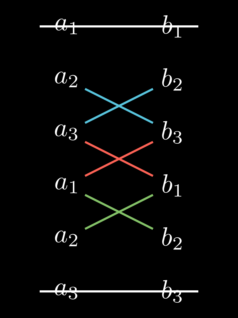
a ⃗ × b ⃗ = ( a 2 b 3 − a 3 b 2 a 3 b 1 − a 1 b 3 a 1 b 2 − a 2 b 1 ) \vec a \times \vec b =
\left(\begin{matrix}
\color{#58C4DD}a_2b_3 - a_3b_2 \\
\color{#FC6255}a_3b_1 - a_1b_3 \\
\color{#83C167}a_1b_2 - a_2b_1
\end{matrix}\right) a × b = a 2 b 3 − a 3 b 2 a 3 b 1 − a 1 b 3 a 1 b 2 − a 2 b 1 Eselsbrücke (siehe Diagramm):
Man schreibt die Vektoren zweimal untereinander. Streicht die erste und letzte Zeile weg. Multipliziert die verbleibenden Werte über Kreuz und bilde die Differenz der Produkte. Satz 💡
Der resultierende Vektor aus a ⃗ × b ⃗ \vec a \times \vec b a × b senkrecht auf a ⃗ \vec a a b ⃗ \vec b b a ⃗ \vec a a b ⃗ \vec b b
Beispiele ( 3 − 5 1 ) × ( − 2 0 4 ) = ( − 5 ⋅ 4 − 1 ⋅ 0 1 ⋅ ( − 2 ) − 3 ⋅ 4 3 ⋅ 0 − ( − 5 ) ⋅ − 2 ) = ( − 20 − 14 − 10 ) \left(\begin{matrix}
3 \\ -5 \\ 1
\end{matrix}\right)
\times
\left(\begin{matrix}
-2 \\ 0 \\ 4
\end{matrix}\right)
=
\left(\begin{matrix}
-5 \cdot 4 - 1 \cdot 0\\
1 \cdot (-2) - 3 \cdot 4 \\
3 \cdot 0 - (-5) \cdot -2
\end{matrix}\right)
=
\left(\begin{matrix}
-20 \\ -14 \\ -10
\end{matrix}\right) 3 − 5 1 × − 2 0 4 = − 5 ⋅ 4 − 1 ⋅ 0 1 ⋅ ( − 2 ) − 3 ⋅ 4 3 ⋅ 0 − ( − 5 ) ⋅ − 2 = − 20 − 14 − 10 ( 2 4 − 1 ) × ( 1 − 3 2 ) = ( 4 ⋅ 2 − ( − 1 ) ⋅ ( − 3 ) ( − 1 ) ⋅ 1 − 2 ⋅ 2 2 ⋅ ( − 3 ) − 4 ⋅ 1 ) = ( 5 − 5 − 10 ) \left(\begin{matrix}
2 \\ 4 \\ -1
\end{matrix}\right)
\times
\left(\begin{matrix}
1 \\ -3 \\ 2
\end{matrix}\right)
=
\left(\begin{matrix}
4 \cdot 2 - (-1) \cdot (-3) \\
(-1) \cdot 1 - 2 \cdot 2 \\
2 \cdot (-3) - 4 \cdot 1\end{matrix}\right)
=
\left(\begin{matrix}
5 \\ -5 \\ -10
\end{matrix}\right) 2 4 − 1 × 1 − 3 2 = 4 ⋅ 2 − ( − 1 ) ⋅ ( − 3 ) ( − 1 ) ⋅ 1 − 2 ⋅ 2 2 ⋅ ( − 3 ) − 4 ⋅ 1 = 5 − 5 − 10 Geradengleichung 💡
Gegeben sind ein Punkt P P P p ⃗ \vec p p u ⃗ ≠ o ⃗ \vec u \neq \vec o u = o P P P u ⃗ \vec u u
g : x ⃗ = p ⃗ + t ⋅ u ⃗ , t ∈ R g: \vec x =
\vec p + t \cdot \vec u, \ t \in \R g : x = p + t ⋅ u , t ∈ R x ⃗ \vec x x g g g p ⃗ \vec p p Stützvektor u ⃗ \vec u u Richtungsvektor t t t Parameter
Gerade durch zwei Punkte aufstellen A = ( 1 ∣ 2 ∣ 1 ) B = ( 3 ∣ 5 ∣ 5 ) A = (1 \, | \, 2 \, | \, 1) \qquad
B = (3 \, | \, 5 \, | \, 5) A = ( 1 ∣ 2 ∣ 1 ) B = ( 3 ∣ 5 ∣ 5 ) g : x ⃗ = O A → + t ⋅ A B → = ( 1 2 1 ) + t ⋅ ( 2 3 4 ) g: \vec x =
\overrightarrow{OA} + t\cdot
\overrightarrow{AB}
=
\left(\begin{matrix}
1 \\ 2 \\ 1
\end{matrix}\right)
+ t \cdot
\left(\begin{matrix}
2 \\ 3 \\ 4
\end{matrix}\right) g : x = O A + t ⋅ A B = 1 2 1 + t ⋅ 2 3 4 Punktprobe Liegt P P P g g g
P ( 3 ∣ 8 ∣ − 3 ) g : x ⃗ = ( 1 2 1 ) + t ⋅ ( 2 3 4 ) P(3 \, | \, 8 \, | -3)
\qquad
g: \vec x =
\left(\begin{matrix}
1 \\ 2 \\ 1
\end{matrix}\right)
+ t \cdot
\left(\begin{matrix}
2 \\ 3 \\ 4
\end{matrix}\right) P ( 3 ∣ 8 ∣ − 3 ) g : x = 1 2 1 + t ⋅ 2 3 4 ( 3 8 − 3 ) = ( 1 2 1 ) + t ⋅ ( 2 3 4 ) ∣ − ( 1 2 1 ) ( 2 6 − 4 ) = t ⋅ ( 2 3 4 ) ⇒ t = 1 ⇒ t = 2 ⇒ t = − 1 ⇒ P liegt nicht auf g \begin{align*}
\left(\begin{matrix}
3 \\ 8 \\ -3
\end{matrix}\right)
&=
\left(\begin{matrix}
1 \\ 2 \\ 1
\end{matrix}\right)
+ t \cdot
\left(\begin{matrix}
2 \\ 3 \\ 4
\end{matrix}\right)
\quad \left|-
\left(\begin{matrix}
1 \\ 2 \\ 1
\end{matrix}\right)\right.
\\
\left(\begin{matrix}
2 \\ 6 \\ -4
\end{matrix}\right)
&=
t \cdot
\left(\begin{matrix}
2 \\ 3 \\ 4
\end{matrix}\right)
\begin{align*}
\Rightarrow t &= 1\\
\Rightarrow t &= 2\\
\Rightarrow t &= -1
\end{align*}
\end{align*}
\\
\boxed{
\Rightarrow P \text{ liegt nicht auf }g
} 3 8 − 3 2 6 − 4 = 1 2 1 + t ⋅ 2 3 4 − 1 2 1 = t ⋅ 2 3 4 ⇒ t ⇒ t ⇒ t = 1 = 2 = − 1 ⇒ P liegt nicht auf g Ebenengleichung: Parametergleichung 💡
Gegeben ist ein Stützvektor p ⃗ \vec p p u ⃗ \vec u u v ⃗ \vec v v Parameterform oder Parametergleichung der Ebene E E E
E : x ⃗ + r ⋅ u ⃗ + s ⋅ v ⃗ r , s ∈ R , u ⃗ ≠ o ⃗ ≠ v ⃗ E: \vec x +
r \cdot \vec u +
s \cdot \vec v
\\
r,s \in \R,
\vec u \neq \vec o \neq \vec v E : x + r ⋅ u + s ⋅ v r , s ∈ R , u = o = v Ebene durch drei Punkte aufstellen A ( 1 ∣ − 1 ∣ 1 ) B ( 1 , 5 ∣ 1 ∣ 0 ) C ( 0 ∣ 1 ∣ 1 ) A(1 \, | -1 \, | \, 1) \qquad
B(1{,}5 \, | \, 1 \, | \ 0) \qquad
C(0 \, | \, 1 \, | \, 1) A ( 1 ∣ − 1 ∣ 1 ) B ( 1 , 5 ∣ 1 ∣ 0 ) C ( 0 ∣ 1 ∣ 1 ) E : x ⃗ = ( 1 − 1 1 ) ⏟ O A → + r ⋅ ( 0 , 5 2 − 1 ) ⏟ A B → + s ⋅ ( − 1 2 0 ) ⏟ A C → E: \vec x =
\underbrace{
\left(\begin{matrix}
1 \\ -1 \\ 1
\end{matrix}\right)
}_{\overrightarrow{OA}}
+ r \cdot
\underbrace{
\left(\begin{matrix}
0{,}5 \\ 2 \\ -1
\end{matrix}\right)
}_{\overrightarrow{AB}}
+ s \cdot
\underbrace{
\left(\begin{matrix}
-1 \\ 2 \\ 0
\end{matrix}\right)
}_{\overrightarrow{AC}} E : x = O A 1 − 1 1 + r ⋅ A B 0 , 5 2 − 1 + s ⋅ A C − 1 2 0 Punktprobe Liegt P P P E E E
P ( 5 ∣ 3 ∣ − 5 ) E : x ⃗ = ( 1 − 1 1 ) + r ⋅ ( 0 , 5 2 − 1 ) + s ⋅ ( − 1 2 0 ) P(5 \, | \, 3 \, | -5)
\qquad
E: \vec x =
\left(\begin{matrix}
1 \\ -1 \\ 1
\end{matrix}\right)
+ r \cdot
\left(\begin{matrix}
0{,}5 \\ 2 \\ -1
\end{matrix}\right)
+ s \cdot
\left(\begin{matrix}
-1 \\ 2 \\ 0
\end{matrix}\right) P ( 5 ∣ 3 ∣ − 5 ) E : x = 1 − 1 1 + r ⋅ 0 , 5 2 − 1 + s ⋅ − 1 2 0 ( 5 3 − 5 ) = ( 1 − 1 1 ) + r ⋅ ( 0 , 5 2 − 1 ) + s ⋅ ( − 1 2 0 ) ∣ − ( 1 − 1 1 ) ( 4 4 − 6 ) = r ⋅ ( 0 , 5 2 − 1 ) + s ⋅ ( − 1 2 0 ) \begin{align*}
\left(\begin{matrix}
5 \\ 3 \\ -5
\end{matrix}\right)
&=
\left(\begin{matrix}
1 \\ -1 \\ 1
\end{matrix}\right)
+ r \cdot
\left(\begin{matrix}
0{,}5 \\ 2 \\ -1
\end{matrix}\right)
+ s \cdot
\left(\begin{matrix}
-1 \\ 2 \\ 0
\end{matrix}\right)
\quad\left |-
\left(\begin{matrix}
1 \\ -1 \\ 1
\end{matrix}\right)
\right.
\\
\left(\begin{matrix}
4 \\ 4 \\ -6
\end{matrix}\right)
&=
r \cdot
\left(\begin{matrix}
0{,}5 \\ 2 \\ -1
\end{matrix}\right)
+ s \cdot
\left(\begin{matrix}
-1 \\ 2 \\ 0
\end{matrix}\right)
\end{align*} 5 3 − 5 4 4 − 6 = 1 − 1 1 + r ⋅ 0 , 5 2 − 1 + s ⋅ − 1 2 0 − 1 − 1 1 = r ⋅ 0 , 5 2 − 1 + s ⋅ − 1 2 0 ⇒ ( 0 , 5 − 1 4 2 2 4 − 1 0 − 6 ) ⇒ s = − 1 ⇒ s = − 4 ⇒ r = 6 ⇒ P liegt nicht auf E \Rightarrow
\left(
\begin{array}{cc|c}
0{,}5 & -1 & 4 \\
2 & 2 & 4 \\
-1 & 0 & -6
\end{array}
\right)
\begin{align*}
\Rightarrow s &= -1 \\
\Rightarrow s &= -4 \\
\Rightarrow r &= 6
\end{align*}
\\
\boxed{
\Rightarrow P \text{ liegt nicht auf } E
} ⇒ 0 , 5 2 − 1 − 1 2 0 4 4 − 6 ⇒ s ⇒ s ⇒ r = − 1 = − 4 = 6 ⇒ P liegt nicht auf E Ebenengleichung: Normalengleichung 💡
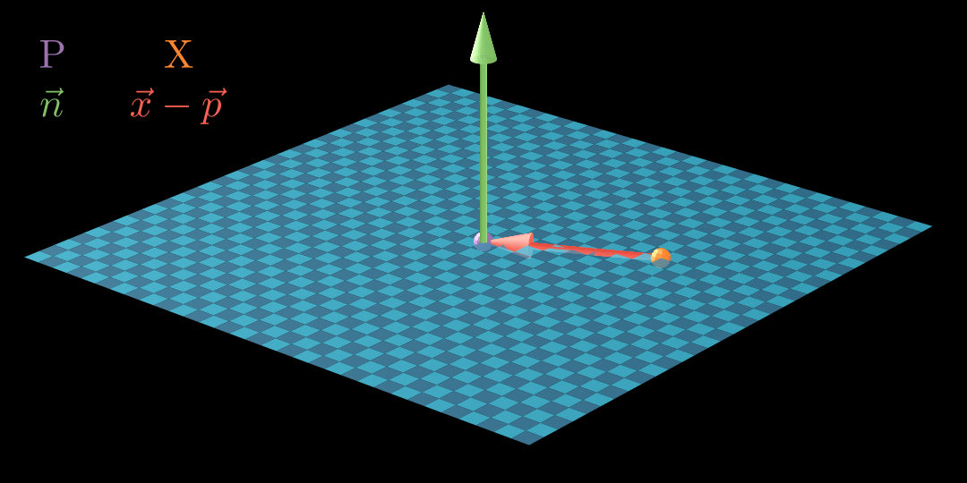
Jede Ebene E E E Normalenvektor n ⃗ \vec n n p ⃗ \vec p p
E : ( x ⃗ − p ⃗ ) ∘ n ⃗ = 0 E:
(\vec x - \vec p)
\circ \vec n = 0 E : ( x − p ) ∘ n = 0 Ebene aufstellen P ( 4 ∣ 1 ∣ 3 ) n ⃗ = ( 2 − 1 5 ) ⇒ E : [ x ⃗ − ( 4 1 3 ) ] ∘ ( 2 − 1 5 ) = 0 P(4 \, | \, 1 \, | \, 3) \qquad
\vec n =
\left(\begin{matrix}
2 \\ -1 \\ 5
\end{matrix}\right)
\\
\Rightarrow
E:
\left[
\vec x -
\left(\begin{matrix}
4 \\ 1 \\ 3
\end{matrix}\right)
\right]
\circ
\left(\begin{matrix}
2 \\ -1 \\ 5
\end{matrix}\right)
= 0 P ( 4 ∣ 1 ∣ 3 ) n = 2 − 1 5 ⇒ E : x − 4 1 3 ∘ 2 − 1 5 = 0 Punktprobe Liegt Q Q Q E E E
Q ( 2 ∣ 1 ∣ 4 ) E : [ x ⃗ − ( 4 1 3 ) ] ∘ ( 2 − 1 5 ) = 0 Q(2 \, | \, 1 \, | \, 4)
\qquad
E:
\left[
\vec x -
\left(\begin{matrix}
4 \\ 1 \\ 3
\end{matrix}\right)
\right]
\circ
\left(\begin{matrix}
2 \\ -1 \\ 5
\end{matrix}\right)
= 0 Q ( 2 ∣ 1 ∣ 4 ) E : x − 4 1 3 ∘ 2 − 1 5 = 0 [ ( 2 1 4 ) − ( 4 1 3 ) ] ∘ ( 2 − 1 5 ) = ? 0 ( − 2 0 1 ) ∘ ( 2 − 1 5 ) = 0 − 2 ⋅ 2 + 0 ⋅ ( − 1 ) + 1 ⋅ 5 = 0 1 ≠ 0 ⇒ P liegt nicht auf E \begin{align*}
\left[
\left(\begin{matrix}
2 \\ 1 \\ 4
\end{matrix}\right)
-
\left(\begin{matrix}
4 \\ 1 \\ 3
\end{matrix}\right)
\right]
\circ
\left(\begin{matrix}
2 \\ -1 \\ 5
\end{matrix}\right)
&\stackrel{?}{=} 0
\\
\left(\begin{matrix}
-2 \\ 0 \\ 1
\end{matrix}\right)
\circ
\left(\begin{matrix}
2 \\ -1 \\ 5
\end{matrix}\right)
&= 0
\\
-2 \cdot 2 +
0 \cdot (-1) +
1 \cdot 5
&= 0
\\
1 &\neq 0
\end{align*}
\\
\boxed{
\Rightarrow P \text{ liegt nicht auf } E
} 2 1 4 − 4 1 3 ∘ 2 − 1 5 − 2 0 1 ∘ 2 − 1 5 − 2 ⋅ 2 + 0 ⋅ ( − 1 ) + 1 ⋅ 5 1 = ? 0 = 0 = 0 = 0 ⇒ P liegt nicht auf E Ebenengleichung: Koordinatengleichung 💡
Jede Ebene E E E Koordinatengleichung beschrieben werden:
E : a x 1 + b x 2 + c x 3 = d E: ax_1 + bx_2 + cx_3 = d E : a x 1 + b x 2 + c x 3 = d Dabei ist ( a b c ) \left(\begin{smallmatrix}
a \\ b \\ c
\end{smallmatrix}\right) ( a b c ) E E E
Ebene durch drei Punkten aufstellen A ( 5 ∣ − 2 ∣ 4 ) B ( − 3 ∣ 0 ∣ 1 ) C ( 3 ∣ 4 ∣ 2 ) A(5 \, | -2 \, | \, 4) \quad
B(-3 \, | \ 0 \, | \, 1) \quad
C(3 \, | \ 4 \, | \, 2) A ( 5 ∣ − 2 ∣ 4 ) B ( − 3 ∣ 0 ∣ 1 ) C ( 3 ∣ 4 ∣ 2 ) A B → = ( − 8 2 − 3 ) A C → = ( − 2 4 − 2 ) A B → × A C → = ( − 8 2 − 3 ) × ( − 2 4 − 2 ) = ( 8 − 10 − 28 ) ⇒ n ⃗ = ( 4 − 5 − 14 ) \overrightarrow{AB} = \left(\begin{matrix}
-8 \\ 2 \\ -3
\end{matrix}\right)
\qquad
\overrightarrow{AC} = \left(\begin{matrix}
-2 \\ 4 \\ -2
\end{matrix}\right)
\\
\overrightarrow{AB} \times \overrightarrow{AC} =
\left(\begin{matrix}
-8 \\ 2 \\ -3
\end{matrix}\right)
\times
\left(\begin{matrix}
-2 \\ 4 \\ -2
\end{matrix}\right)
=
\left(\begin{matrix}
8 \\ -10 \\ -28
\end{matrix}\right)
\quad\Rightarrow
\vec n =
\left(\begin{matrix}
4 \\ -5 \\ -14
\end{matrix}\right) A B = − 8 2 − 3 A C = − 2 4 − 2 A B × A C = − 8 2 − 3 × − 2 4 − 2 = 8 − 10 − 28 ⇒ n = 4 − 5 − 14 ❗
Probe machen: n ⃗ ∘ A B → = 0 \color{df5441}\vec n \circ \overrightarrow{AB} = 0 n ∘ A B = 0 und n ⃗ ∘ A C → = 0 \color{df5441}\vec n \circ \overrightarrow{AC} = 0 n ∘ A C = 0 .
E : 4 x 1 − 5 x 2 − 14 x 3 = − 26 ⏟ NR (B eingesetzt): 4 ⋅ ( − 3 ) − 5 ⋅ 0 − 14 ⋅ 1 = − 26 E: 4x_1-5x_2-14x_3=
\underbrace{-26}
\\
\text{NR (B eingesetzt): }
4 \cdot (-3) -
5 \cdot 0 -
14 \cdot 1 = -26 E : 4 x 1 − 5 x 2 − 14 x 3 = − 26 NR (B eingesetzt): 4 ⋅ ( − 3 ) − 5 ⋅ 0 − 14 ⋅ 1 = − 26 Punktprobe Liegt P P P E E E
P ( 3 ∣ 2 ∣ 2 ) E : 4 x 1 − 5 x 2 − 14 x 3 = − 26 P(3 \ | \ 2 \ | \ 2) \quad
E: 4x_1 - 5x_2 - 14x_3 = -26 P ( 3 ∣ 2 ∣ 2 ) E : 4 x 1 − 5 x 2 − 14 x 3 = − 26 4 ⋅ 3 − 5 ⋅ 2 − 14 ⋅ 2 = ? − 26 − 26 = − 26 ⇒ P liegt auf E \begin{align*}
4 \cdot 3 -
5 \cdot 2 -
14 \cdot 2
&\stackrel{?}{=} -26
\\
-26 &= -26
\end{align*}
\\
\boxed{
\Rightarrow P \text{ liegt auf }E
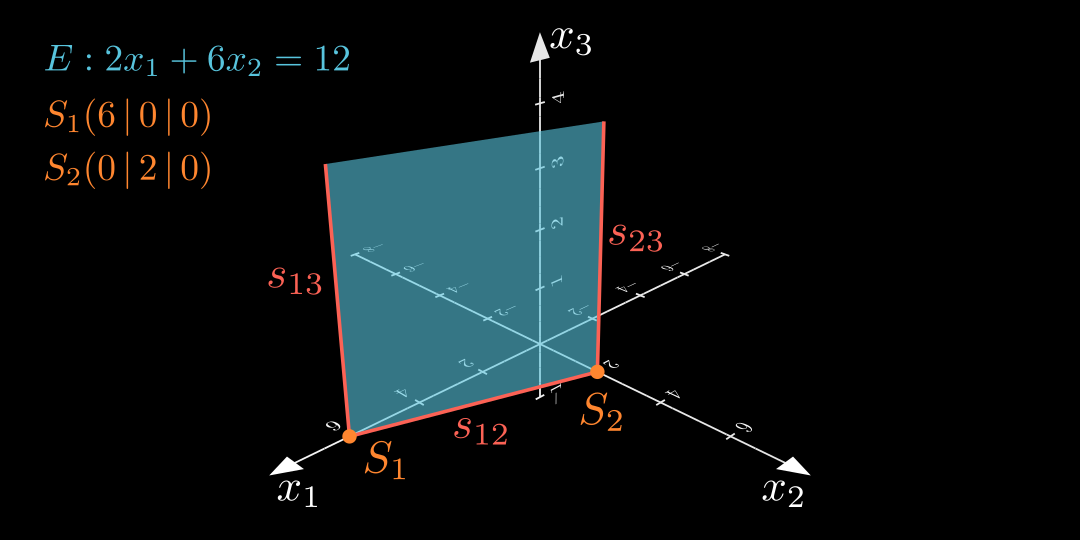
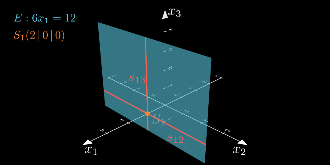
} 4 ⋅ 3 − 5 ⋅ 2 − 14 ⋅ 2 − 26 = ? − 26 = − 26 ⇒ P liegt auf E Spurpunkte und Spurgeraden 💡
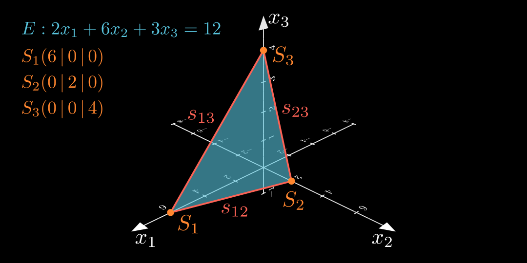
Um eine Ebene in einem Koordinatensystem zu veranschaulichen, zeichnet man einen Ausschnitt der Ebene. Dabei orientiert man sich an den jeweiligen Schnittpunkten der Ebene mit den Koordinatenachsen. Diese Punkte heißen Spurpunkte .
💡
Die Gesamtheit aller Schnittpunkte einer Ebene mit einer Koordinatenebene heißen Spurgerade .
In den folgenden Beispielen sind stets alle Spurpunkte \color{#FF862F} \text{Spurpunkte} Spurpunkte Spurgeraden \color{#FC6255}\text{Spurgeraden} Spurgeraden
Achsenabschnittsform 💡
Wenn man alle Spurpunkte einer Ebene kennt, die nicht durch den Ursprung verläuft, so kann man direkt deren Achsenabschnittsform (eine spezielle Koordinatengleichung) anlegen.
Beispiel S 1 ( 5 ∣ 0 ∣ 0 ) S 2 ( 0 ∣ − 2 ∣ 0 ) S 3 ( 0 ∣ 0 ∣ 0 , 5 ) S_1 (5 \, | \, 0 \, | \, 0) \quad
S_2 (0 \, | -2 \, | \, 0) \quad
S_3 (0 \, | \, 0 \, | \, 0{,}5) S 1 ( 5 ∣ 0 ∣ 0 ) S 2 ( 0 ∣ − 2 ∣ 0 ) S 3 ( 0 ∣ 0 ∣ 0 , 5 ) ⇒ E : 1 5 x 1 − 1 2 x 2 + 2 x 3 = 1 ∣ ⋅ 10 E : 2 x 1 − 5 x 2 + 20 x 3 = 10 \begin{align*}
\Rightarrow
E: \frac 15 x_1 -
\frac12 x_2 + 2x_3 &= 1
\quad | \cdot 10
\\
E: 2x_1 - 5x_2 + 20x_3 &= 10
\end{align*} ⇒ E : 5 1 x 1 − 2 1 x 2 + 2 x 3 E : 2 x 1 − 5 x 2 + 20 x 3 = 1 ∣ ⋅ 10 = 10 Gegenseitige Lage von Ebenen und Geraden 💡
Wenn der Normalenvektor der Ebene ein Vielfaches des Richtungsvektors ist, so schneidet die Gerade die Ebene orthogonal. Wenn das Skalarprodukt von Normalenvektor der Ebene und Richtungsvektor der Geraden 0 ist, so ist die Gerade in der Ebene enthalten, wenn der Stützvektor in der Ebene enthalten ist. Ist der Stützvektor nicht in der Ebene enthalten, so ist die Gerade parallel zur Ebene. Ansonsten und in Fall 1 gibt es genau einen Schnittpunkt (Durchstoßpunkt ). Durchstoßpunkt berechnen E : x 1 − x 2 + 2 x 3 = 9 g : x ⃗ = ( 3 2 0 ) + t ⋅ ( − 2 2 3 ) E: x_1 -x_2 + 2x_3 = 9 \qquad
g: \vec x =
\left(\begin{matrix}
3 \\ 2 \\ 0
\end{matrix}\right)
+
t \cdot
\left(\begin{matrix}
-2 \\ 2 \\ 3
\end{matrix}\right)
\qquad E : x 1 − x 2 + 2 x 3 = 9 g : x = 3 2 0 + t ⋅ − 2 2 3 Schneide E & g ( g in E einsetzen): ( 3 − 2 t ) − ( 2 + 2 t ) + 2 ⋅ ( 0 + 3 t ) = 9 1 + 2 t = 9 ∣ − 1 ∣ : 2 t = 4 t = 4 in g einsetzen: ⇒ S ( − 5 ∣ 10 ∣ 12 ) \text{Schneide } E \text{ \& } g
\text{ (} g \text{ in } E \text{ einsetzen): }
\\
\begin{align*}
(3-2t) - (2+2t) +
2 \cdot (0 + 3t) &= 9
\\
1 + 2t &= 9
\quad
| -1 \quad |:2
\\
t &= 4
\end{align*}
\\
t=4 \text{ in } g \text{ einsetzen:}
\\
\boxed{
\Rightarrow
S(-5 \, | \, 10 \, | 12)
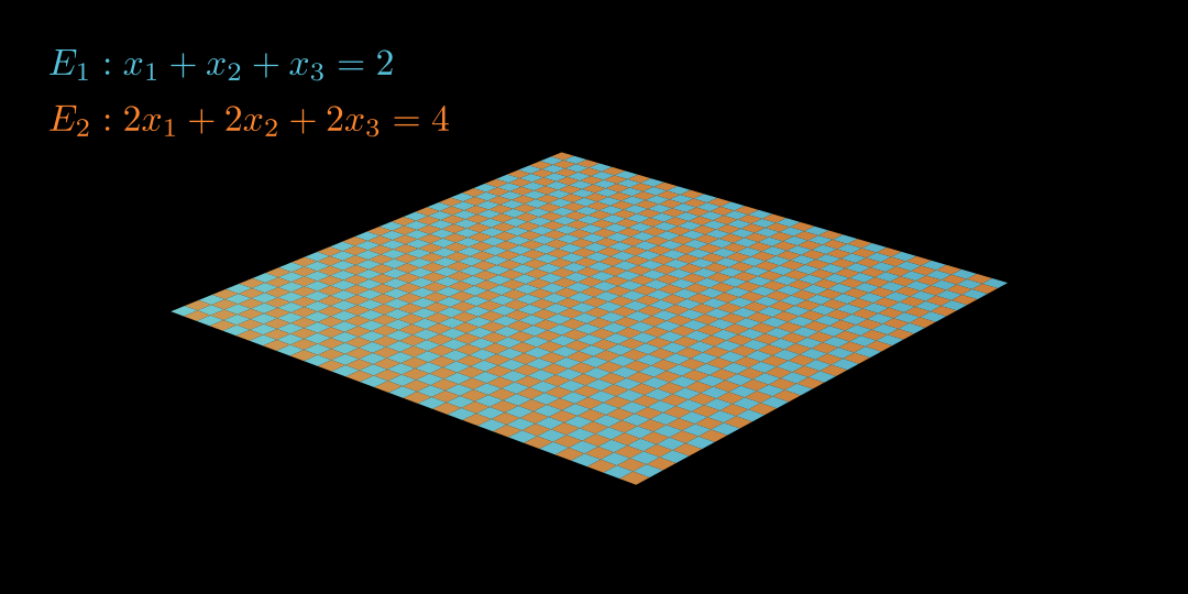
} Schneide E & g ( g in E einsetzen): ( 3 − 2 t ) − ( 2 + 2 t ) + 2 ⋅ ( 0 + 3 t ) 1 + 2 t t = 9 = 9 ∣ − 1 ∣ : 2 = 4 t = 4 in g einsetzen: ⇒ S ( − 5 ∣ 10 ∣12 ) Gegenseitige Lage von Ebenen Identisch Normalenvektoren und Koordinatengleichungen sind Vielfache voneinander.
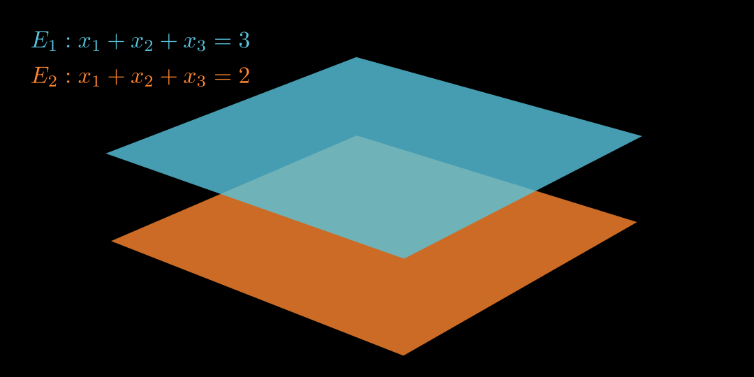
Parallel Normalenvektoren sind Vielfache voneinander, aber Koordinatengleichungen sind keine vielfache voneinander.
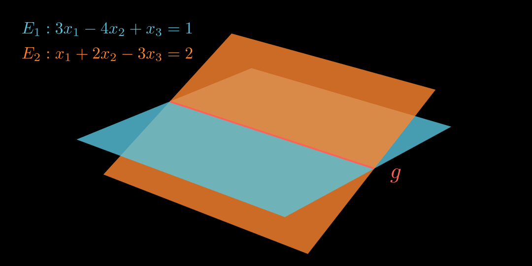
Schneidend Schnittgerade bestimmen E 1 : 3 x 1 − 4 x 2 + x 3 = 1 E 2 : x 1 + 2 x 2 − 3 x 3 = 2 E_1: 3x_1 - 4x_2 + x_3 = 1 \\
E_2: x_1 + 2x_2 - 3x_3 = 2 E 1 : 3 x 1 − 4 x 2 + x 3 = 1 E 2 : x 1 + 2 x 2 − 3 x 3 = 2 Unterbestimmtes LGS: I) II) I − 3 I I ) 3 x 1 − 4 x 2 + x 3 = 1 x 1 + 2 x 2 − 3 x 3 = 2 x 1 − 10 x 2 + 10 x 3 = 5 \text{Unterbestimmtes LGS:}
\\
\begin{align*}
\textit{I) } \ \\
\textit{II) } \ \\
\textit{I } -3 {II) } \
\end{align*}
\begin{alignat*} {5}
3 &x_1 - &4 &x_2 + &&x_3 = 1 \\
&x_1 + &2 &x_2 - & 3 &x_3 = 2 \\
&\phantom{x_1} - &10 &x_2 + &10 &x_3 = 5
\end{alignat*} Unterbestimmtes LGS: I) II) I − 3 II ) 3 x 1 − x 1 + x 1 − 4 2 10 x 2 + x 2 − x 2 + 3 10 x 3 = 1 x 3 = 2 x 3 = 5 W a ¨ hle x 3 = t : ⇒ x 2 = − 1 2 + t ⇒ x 1 = 3 + t ⇒ g : x ⃗ = ( 3 − 1 2 0 ) + t ⋅ ( 1 1 1 ) \text{Wähle } x_3 = t:
\quad
\begin{align*}
\Rightarrow x_2 &= -\frac12 + t\\
\Rightarrow x_1 &= 3 + t
\end{align*}
\\
\boxed{
\Rightarrow g: \vec x =
\left(\begin{matrix}
3 \\ -\frac12 \\ 0
\end{matrix}\right)
+
t \cdot
\left(\begin{matrix}
1 \\ 1 \\ 1
\end{matrix}\right)
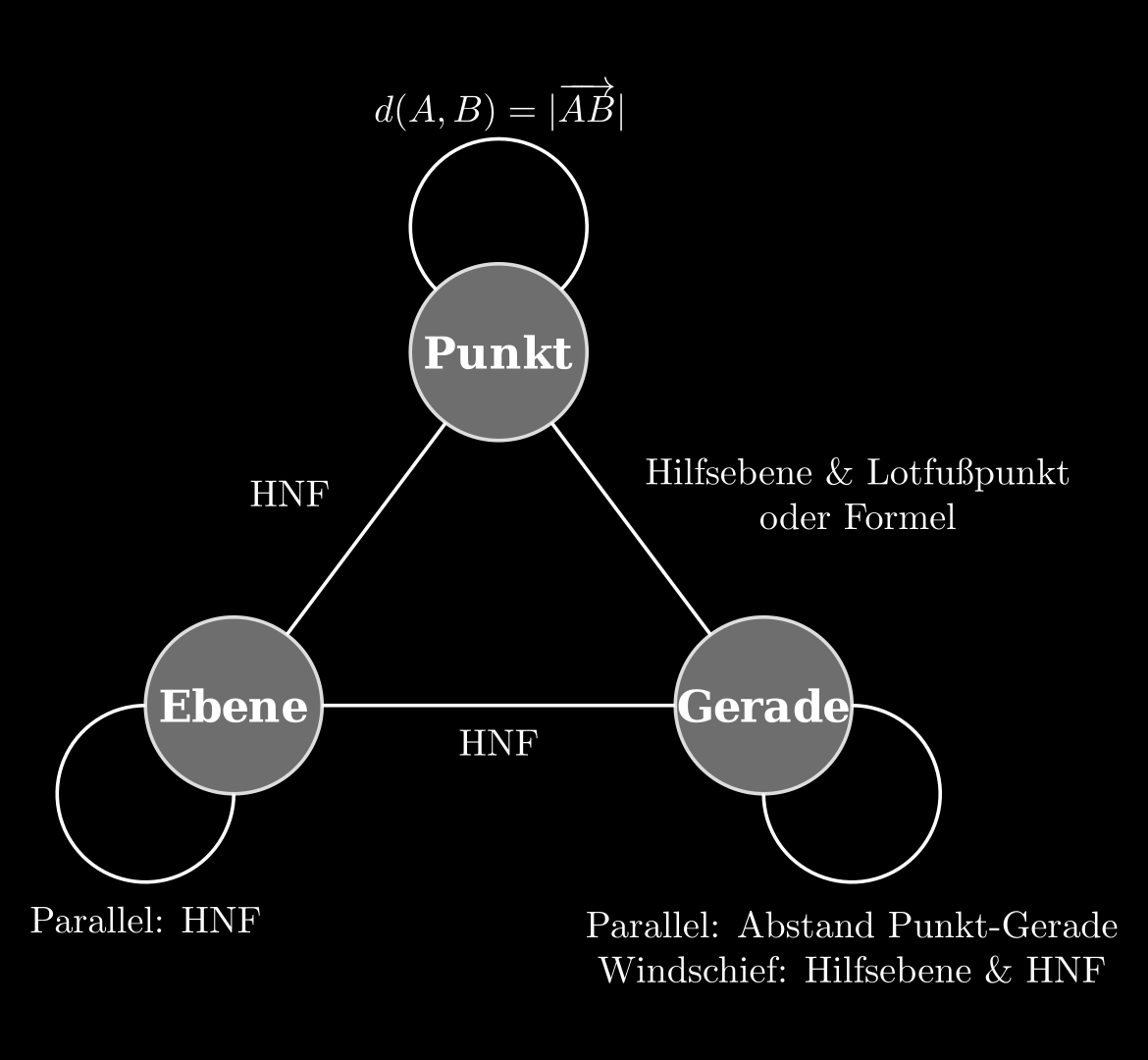
} W a ¨ hle x 3 = t : ⇒ x 2 ⇒ x 1 = − 2 1 + t = 3 + t ⇒ g : x = 3 − 2 1 0 + t ⋅ 1 1 1 Abstandsberechnungen (Übersicht) 💡
Hesse’sche Normal(en)form (HNF) 💡
Eine Ebenengleichung E : ( x ⃗ − p ⃗ ) ∘ n ⃗ 0 = 0 E: (\vec x - \vec p) \circ \vec n_0 = 0 E : ( x − p ) ∘ n 0 = 0 Hesse’sche Normal(en)form (HNF) von E E E n ⃗ 0 \vec n_0 n 0 Einheitsnormalenvektor .
Der Abstand d ( E , Q ) d(E, Q) d ( E , Q ) E E E Q Q Q
d ( E , Q ) = ∣ ( q ⃗ − p ⃗ ) ∘ n ⃗ 0 ∣ d(E, Q) = |(\vec q - \vec p)\circ\vec n_0| d ( E , Q ) = ∣ ( q − p ) ∘ n 0 ∣ 💡
Für die Koordinatengleichung von E : a 1 x 1 + a 2 x 2 + a 3 x 3 = b E:a_1x_1+a_2x_2+a_3x_3=b E : a 1 x 1 + a 2 x 2 + a 3 x 3 = b
d ( E , Q ) = ∣ a 1 x 1 + a 2 x 2 + a 3 x 3 − b ∣ a 1 2 + a 2 2 + a 3 2 d(E, Q) = \frac {
|a_1x_1+a_2x_2+a_3x_3-b|
}{
\sqrt{{a_1}^2+{a_2}^2+{a_3}^2}
} d ( E , Q ) = a 1 2 + a 2 2 + a 3 2 ∣ a 1 x 1 + a 2 x 2 + a 3 x 3 − b ∣ Beispiele Normalenform:
E : [ x ⃗ − ( 9 − 8 6 ) ] ∘ ( 2 2 1 ) = 0 P ( 1 ∣ − 1 ∣ 0 ) E:
\left[
\vec x
-
\left(\begin{matrix}
9 \\ -8 \\ 6
\end{matrix}\right)
\right]
\circ
\left(\begin{matrix}
2 \\ 2 \\ 1
\end{matrix}
\right)
= 0
\qquad
P(1 \, | \, {-1} \, | \, 0) E : x − 9 − 8 6 ∘ 2 2 1 = 0 P ( 1 ∣ − 1 ∣ 0 ) d ( E , P ) = ∣ ( 0 − 1 1 ) − ( 9 − 8 6 ) ∘ ( 2 2 1 ) ∣ ⋅ 1 3 ⏟ n ⃗ 0 = ∣ ( − 9 7 − 5 ) ∘ ( 2 2 1 ) ∣ ⋅ 1 3 = 9 ⋅ 1 3 = 3 d(E, P) = \left|
\left(\begin{matrix}
0 \\ -1 \\ 1
\end{matrix}\right)
-
\left(\begin{matrix}
9 \\ -8 \\ 6
\end{matrix}\right)
\circ
\right.
\underbrace{
\left.
\left(\begin{matrix}
2 \\ 2 \\ 1
\end{matrix}\right)
\right|
\cdot\frac13
}_{\vec n_0} =
\left|
\left(\begin{matrix}
-9 \\ 7 \\ -5
\end{matrix}\right)
\circ
\left(\begin{matrix}
2 \\ 2 \\ 1
\end{matrix}\right)
\right|
\cdot\frac13
=
9 \cdot \frac 13 =3 d ( E , P ) = 0 − 1 1 − 9 − 8 6 ∘ n 0 2 2 1 ⋅ 3 1 = − 9 7 − 5 ∘ 2 2 1 ⋅ 3 1 = 9 ⋅ 3 1 = 3 Koordinatenform:
F : 2 x 1 − 4 x 2 + 4 x 3 = 2 Q ( 4 ∣ 2 ∣ 5 ) F: 2x_1-4x_2+4x_3 = 2 \qquad
Q(4 \, | \, 2 \, | \, 5) F : 2 x 1 − 4 x 2 + 4 x 3 = 2 Q ( 4 ∣ 2 ∣ 5 ) d ( F , Q ) = ∣ 2 ⋅ 4 − 4 ⋅ 2 + 4 ⋅ 5 − 2 ∣ 2 2 + 4 2 + 4 2 = ∣ 18 ∣ 36 = 3 d(F,Q) = \frac{
|2 \cdot 4 - 4 \cdot 2 +
4 \cdot 5 - 2|
}{
\sqrt{2^2+4^2+4^2}
}
=
\frac{|18|}{\sqrt{36}}
=
3 d ( F , Q ) = 2 2 + 4 2 + 4 2 ∣2 ⋅ 4 − 4 ⋅ 2 + 4 ⋅ 5 − 2∣ = 36 ∣18∣ = 3 Abstand Punkt-Ebene 💡
Unter dem Abstand d d d P P P E E E P P P E E E
Beispiel E : x 1 + 8 x 2 − 4 x 3 = 25 P ( 2 ∣ 0 ∣ 1 ) E: x_1 + 8x_2 -4x_3 = 25 \qquad
P(2 \, | \, 0 \, | \, 1) E : x 1 + 8 x 2 − 4 x 3 = 25 P ( 2 ∣ 0 ∣ 1 ) Variante 1: HNF d ( E , P ) = ∣ 2 − 4 − 25 ∣ 1 2 + 8 2 + 4 2 = ∣ − 27 ∣ 81 = 27 9 = 3 d(E, P) = \frac{
|2-4-25|
}{
\sqrt{1^2+8^2+4^2}
}
=
\frac{|{-27}|}{\sqrt{81}}
=
\frac{27}{9}=3 d ( E , P ) = 1 2 + 8 2 + 4 2 ∣2 − 4 − 25∣ = 81 ∣ − 27 ∣ = 9 27 = 3 Variante 2: Durchstoßpunkt Hilfsgerade g durch P in Richtung des Normalenvektors g : x ⃗ = ( 2 0 1 ) + r ⋅ ( 1 8 − 4 ) \text{Hilfsgerade }g \text{ durch }P \text{ in Richtung des Normalenvektors} \\
g: \vec x =
\left(\begin{matrix}
2 \\ 0 \\ 1
\end{matrix}\right)
+ r \cdot \left(\begin{matrix}
1 \\ 8 \\ -4
\end{matrix}\right) Hilfsgerade g durch P in Richtung des Normalenvektors g : x = 2 0 1 + r ⋅ 1 8 − 4 E & g schneiden um Lotfußpunkt zu bestimmen 2 + r + 8 ⋅ 8 r − 4 ⋅ ( 1 − 4 r ) = 25 ⇒ r = 1 3 ⇒ F ( 7 3 ∣ 8 3 ∣ − 1 3 ) E \text{ \& } g \text{ schneiden um Lotfußpunkt zu bestimmen} \\
\begin{align*}
2+r + 8 \cdot 8r -
4 \cdot (1-4r) &= 25
\\
\Rightarrow r &= \frac13
\end{align*}
\\\Rightarrow
F\left(
\frac73 \, \left| \,
\frac83 \, \right|
{-\frac13}
\right) E & g schneiden um Lotfußpunkt zu bestimmen 2 + r + 8 ⋅ 8 r − 4 ⋅ ( 1 − 4 r ) ⇒ r = 25 = 3 1 ⇒ F ( 3 7 3 8 − 3 1 ) d ( E , P ) = d ( F , P ) = ∣ F R → ∣ = ∣ ( 2 0 1 ) − ( 7 3 8 3 − 1 3 ) ∣ = ( 1 3 ) 2 + ( 8 3 ) 2 + ( 4 3 ) 2 = 9 = 3 \begin{align*}
d(E,P) = d(F,P) =
|\overrightarrow{FR}| &=
\left|
\left(\begin{matrix}
2 \\ 0 \\ 1
\end{matrix}\right)
-
\left(\begin{matrix}
\frac73 \\ \frac83 \\ -\frac13
\end{matrix}\right)
\right|
\\
&=\sqrt{
\left(\frac13\right)^2 +
\left(\frac83\right)^2 +
\left(\frac43\right)^2
}
=
\sqrt9 = 3
\end{align*} d ( E , P ) = d ( F , P ) = ∣ FR ∣ = 2 0 1 − 3 7 3 8 − 3 1 = ( 3 1 ) 2 + ( 3 8 ) 2 + ( 3 4 ) 2 = 9 = 3 Abstand Punkt-Gerade 💡
Algorithmus Stelle Hilfsebene H H H P P P g g g Erhalte Punkt F F F g g g H H H d ( R , g ) = ∣ F R → ∣ d(R, g) = |\overrightarrow{FR}| d ( R , g ) = ∣ FR ∣ 💡
Formel Für den Abstand eines Punktes R R R g : x ⃗ = p ⃗ + s ⋅ u ⃗ g: \vec x = \vec p + s \cdot \vec u g : x = p + s ⋅ u
d ( R , g ) = ∣ P R → × u ⃗ 0 ∣ d(R, g) = |\overrightarrow{PR} \times \vec u_0| d ( R , g ) = ∣ PR × u 0 ∣ Beispiel g : x ⃗ = ( 4 3 1 ) + s ⋅ ( 2 1 − 2 ) R ( 2 ∣ − 3 ∣ 5 ) g: \vec x =
\left(\begin{matrix}
4 \\ 3 \\ 1
\end{matrix}\right)
+ s \cdot
\left(\begin{matrix}
2 \\ 1 \\ -2
\end{matrix}\right)
\qquad
R(2 \, | {-3} \, | \,5) g : x = 4 3 1 + s ⋅ 2 1 − 2 R ( 2 ∣ − 3 ∣ 5 ) Variante 1: Algorithmus 1. Hilfsebene aufstellen ⇒ H : 2 x 1 + x 2 − 2 x 3 = − 9 NR: 2 ⋅ 2 + ( − 3 ) − 2 ⋅ 5 = − 9 \text{1. Hilfsebene aufstellen} \\
\Rightarrow H: 2x_1 +x_2 -2x_3 = -9
\qquad
\text{NR: }
2\cdot2 + (-3) - 2 \cdot 5 = -9
1. Hilfsebene aufstellen ⇒ H : 2 x 1 + x 2 − 2 x 3 = − 9 NR: 2 ⋅ 2 + ( − 3 ) − 2 ⋅ 5 = − 9 2. Schnittpunkt bestimmen 2 ⋅ ( 4 + 2 s ) + 3 + s − 2 ⋅ ( 1 − 2 s ) = − 9 9 + 9 s = − 9 ∣ − 9 ∣ : 9 s = − 2 ⇒ F ( 0 ∣ 1 ∣ 5 ) \text{2. Schnittpunkt bestimmen}\\
\begin{align*}
2 \cdot (4+2s) + 3 + s -
2 \cdot (1 - 2s)
&= -9 \\
9+9s &= -9 \quad |-9 \ |:9 \\
s &= -2
\end{align*}
\\
\Rightarrow
F(0 \, | \, 1 \, | \,5) 2. Schnittpunkt bestimmen 2 ⋅ ( 4 + 2 s ) + 3 + s − 2 ⋅ ( 1 − 2 s ) 9 + 9 s s = − 9 = − 9 ∣ − 9 ∣ : 9 = − 2 ⇒ F ( 0 ∣ 1 ∣ 5 ) 3. Abstand berechnen d ( R , g ) = d ( R , F ) = ∣ R F → ∣ = 2 2 + 4 2 + 0 2 = 20 \text{3. Abstand berechnen}\\
d(R, g) = d(R, F) = |\overrightarrow{RF}| =
\sqrt{2^2+4^2+0^2}=\sqrt{20} 3. Abstand berechnen d ( R , g ) = d ( R , F ) = ∣ RF ∣ = 2 2 + 4 2 + 0 2 = 20 Variante 2: Formel R P → = ( 2 6 − 4 ) ∣ u ⃗ ∣ = 3 ⇒ u ⃗ 0 = 1 3 ⋅ ( 2 1 − 2 ) \overrightarrow{RP} =
\left(\begin{matrix}
2 \\ 6 \\ -4
\end{matrix}\right)
\qquad
|\vec u| = 3
\ \ \Rightarrow \ \
\vec u_0 =
\frac1{3} \cdot
\left(\begin{matrix}
2 \\ 1 \\ -2
\end{matrix}\right) RP = 2 6 − 4 ∣ u ∣ = 3 ⇒ u 0 = 3 1 ⋅ 2 1 − 2 d ( R , g ) = ∣ R P → × u ⃗ 0 ∣ = ∣ ( 2 6 − 4 ) × ( 2 1 − 2 ) ∣ ⋅ 1 3 ⏟ u ⃗ 0 = ∣ ( − 8 − 4 − 10 ) ∣ ⋅ 1 3 = 180 ⋅ 1 9 = 20 \begin{align*}
d(R, g) =
|\overrightarrow{RP}
\times \vec u_0| &=
\left|
\left(\begin{matrix}
2 \\ 6 \\ -4
\end{matrix}\right)
\times
\right.
\underbrace{
\left.
\left(\begin{matrix}
2 \\ 1 \\ -2
\end{matrix}\right)
\right|
\cdot \frac 13
}_{\vec u_0}\\
&=
\left|
\left(\begin{matrix}
-8 \\ -4 \\ -10
\end{matrix}\right)
\right|
\cdot \frac 13
=\sqrt{180}\cdot\sqrt{\frac19}
=\sqrt{20}
\end{align*} d ( R , g ) = ∣ RP × u 0 ∣ = 2 6 − 4 × u 0 2 1 − 2 ⋅ 3 1 = − 8 − 4 − 10 ⋅ 3 1 = 180 ⋅ 9 1 = 20 Abstand Gerade-Gerade (Parallel) 💡
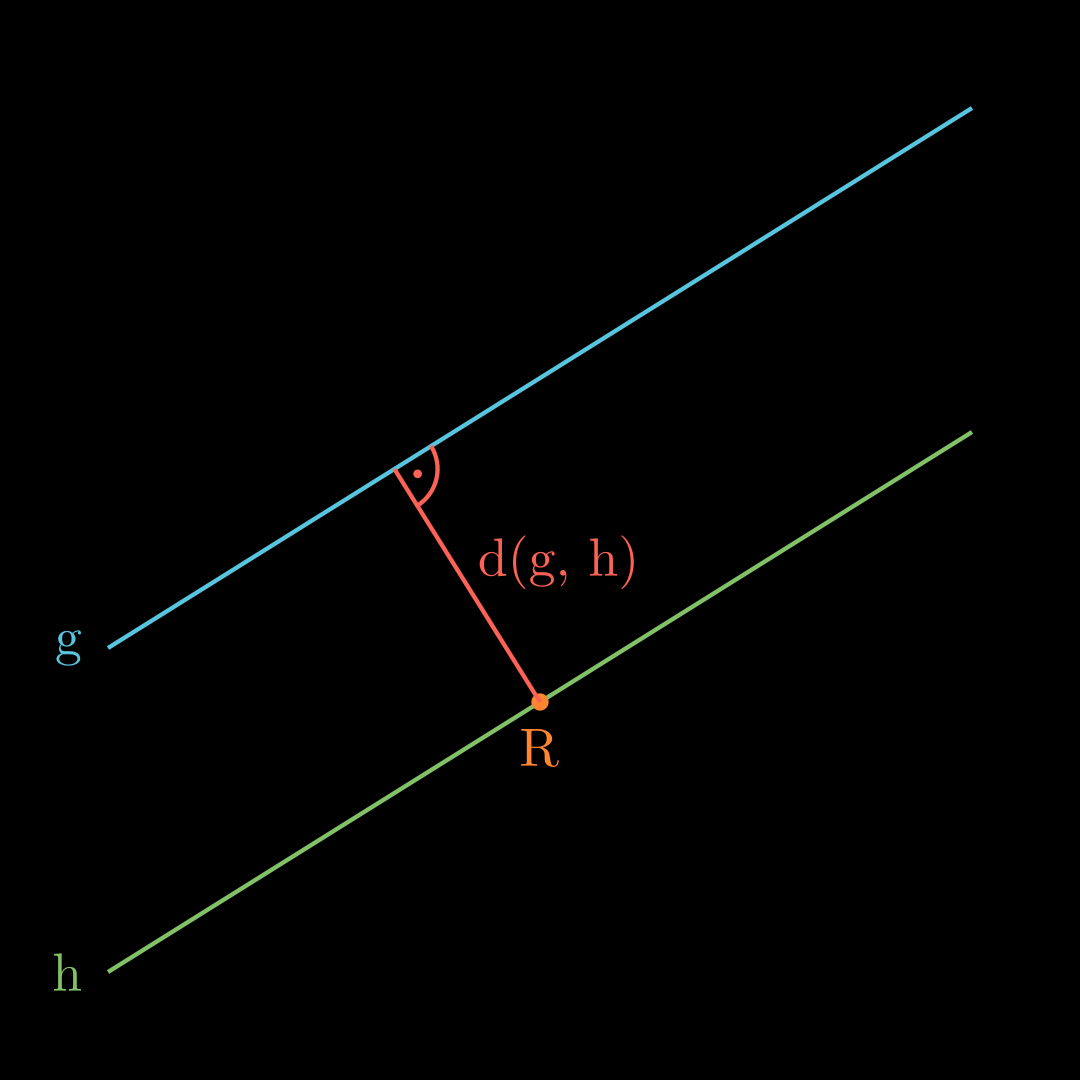
Um den Abstand zwei paralleler Geraden g g g h h h R R R h h h g g g
d ( g , h ) = d ( g , R ) d(g, h) = d(g,R) d ( g , h ) = d ( g , R ) Beispiel Siehe Beispiel Abstand Punkt-Gerade.
Abstand Gerade-Gerade (Windschief) 💡
Gegeben sind die Geraden g : x ⃗ = p ⃗ + r ⋅ u ⃗ g: \vec x = \vec p + r \cdot \vec u g : x = p + r ⋅ u h : x ⃗ = q ⃗ + s ⋅ v ⃗ h: \vec x = \vec q + s \cdot \vec v h : x = q + s ⋅ v
Stelle eine Hilfsebene E E E n ⃗ = u ⃗ × v ⃗ \vec n = \vec u \times \vec v n = u × v P P P E E E h h h g g g d ( g , h ) = d ( E , h ) = d ( E , Q ) ⏟ HNF d(g, h) = d(E, h) = \underbrace{d(E, Q)}_{\text{HNF}} d ( g , h ) = d ( E , h ) = HNF d ( E , Q ) ODER
d ( g , h ) = ∣ ( q ⃗ − p ⃗ ) ∘ n ⃗ 0 ∣ d(g, h) = \left | (\vec q - \vec p) \circ \vec n_0 \right | d ( g , h ) = ∣ ( q − p ) ∘ n 0 ∣
Beispiel g : x ⃗ = ( 9 − 8 6 ) + r ⋅ ( 2 − 3 2 ) h : x ⃗ = ( 6 5 4 ) + s ⋅ ( 1 − 1 0 ) g: \vec x =
\left(\begin{matrix}
9 \\ -8 \\ 6
\end{matrix}\right)
+ r \cdot
\left(\begin{matrix}
2 \\ -3 \\ 2
\end{matrix}\right)
\qquad
h: \vec x =
\left(\begin{matrix}
6 \\ 5 \\ 4
\end{matrix}\right)
+ s \cdot
\left(\begin{matrix}
1 \\ -1 \\ 0
\end{matrix}\right) g : x = 9 − 8 6 + r ⋅ 2 − 3 2 h : x = 6 5 4 + s ⋅ 1 − 1 0 n ⃗ = ( 2 − 3 2 ) × ( 1 − 1 0 ) = ( 2 2 1 ) ∣ n ⃗ ∣ = 3 \vec n =
\left(\begin{matrix}
2 \\ -3 \\ 2
\end{matrix}\right)
\times
\left(\begin{matrix}
1 \\ -1 \\ 0
\end{matrix}\right)
=
\left(\begin{matrix}
2 \\ 2 \\ 1
\end{matrix}\right)
\qquad
|\vec n| =3 n = 2 − 3 2 × 1 − 1 0 = 2 2 1 ∣ n ∣ = 3 d ( E , Q ) = ∣ ( 6 5 4 ) − ( 9 − 8 6 ) ∘ ( 2 2 1 ) ∣ ⋅ 1 3 ⏟ n ⃗ 0 = ∣ ( − 3 13 − 2 ) ∘ ( 2 2 1 ) ∣ ⋅ 1 3 = 18 ⋅ 1 3 = 6 d(E, Q) = \left|
\left(\begin{matrix}
6 \\ 5 \\ 4
\end{matrix}\right)
-
\left(\begin{matrix}
9 \\ -8 \\ 6
\end{matrix}\right)
\circ
\right.
\underbrace{
\left.
\left(\begin{matrix}
2 \\ 2 \\ 1
\end{matrix}\right)
\right|
\cdot\frac13
}_{\vec n_0} =
\left|
\left(\begin{matrix}
-3 \\ 13 \\ -2
\end{matrix}\right)
\circ
\left(\begin{matrix}
2 \\ 2 \\ 1
\end{matrix}\right)
\right|
\cdot\frac13
=
18 \cdot \frac 13 = 6 d ( E , Q ) = 6 5 4 − 9 − 8 6 ∘ n 0 2 2 1 ⋅ 3 1 = − 3 13 − 2 ∘ 2 2 1 ⋅ 3 1 = 18 ⋅ 3 1 = 6 ODER
d ( g , h ) = ∣ ( ( 6 5 4 ) − ( 9 − 8 6 ) ) ∘ 1 3 ⋅ ( 2 2 1 ) ⏟ n ⃗ 0 ∣ = ∣ ( − 3 13 − 2 ) ∘ ( 2 3 2 3 1 3 ) ∣ = 6 d(g, h) = \left|
\left(
\left(\begin{matrix}
6 \\ 5 \\ 4
\end{matrix}\right)
-
\left(\begin{matrix}
9 \\ -8 \\ 6
\end{matrix}\right)
\right)
\circ
\underbrace {
\frac13 \cdot
\left(\begin{matrix}
2 \\ 2 \\ 1
\end{matrix}\right)
}_{\vec n_0}
\right|
=
\left|
\left(\begin{matrix}
-3 \\ 13 \\ -2
\end{matrix}\right)
\circ
\left(\begin{matrix}
\frac23 \\ \frac23 \\ \frac13
\end{matrix}\right)
\right|
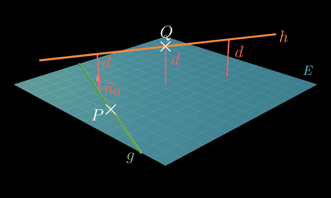
=6 d ( g , h ) = 6 5 4 − 9 − 8 6 ∘ n 0 3 1 ⋅ 2 2 1 = − 3 13 − 2 ∘ 3 2 3 2 3 1 = 6 Abstand Gerade-Ebene (Parallel) 💡
Um den Abstand der Ebene E E E g g g Q Q Q g g g
d ( E , g ) = d ( E , Q ) ⏟ HNF d(E, g) =
\underbrace{d(E, Q)}
_{\text{HNF}} d ( E , g ) = HNF d ( E , Q ) Beispiel E : x 1 + 2 x 2 − 2 x 3 = 4 g : x ⃗ = ( 4 2 1 ) + t ⋅ ( 0 1 1 ) E: x_1 + 2x_2 - 2x_3 = 4
\qquad
g: \vec x =
\left(\begin{matrix}
4 \\ 2 \\ 1
\end{matrix}\right)
+ t \cdot
\left(\begin{matrix}
0 \\ 1 \\ 1
\end{matrix}\right) E : x 1 + 2 x 2 − 2 x 3 = 4 g : x = 4 2 1 + t ⋅ 0 1 1 d ( E , g ) = d ( E , ( 4 ∣ 2 ∣ 1 ) ) = ∣ 4 + 4 − 2 − 4 ∣ 3 = 2 3 d(E, g) =
d(E, (4 \, | \, 2 \, | \, 1)) =
\frac{|4+4-2-4|}{3} = \frac23 d ( E , g ) = d ( E , ( 4 ∣ 2 ∣ 1 )) = 3 ∣4 + 4 − 2 − 4∣ = 3 2 Abstand Ebene-Ebene (Parallel) 💡
Um den Abstand der parallelen Ebenen E E E F F F P P P F F F
d ( E , F ) = d ( E , P ) ⏟ HNF d(E, F) =
\underbrace{d(E, P)}
_{\text{HNF}} d ( E , F ) = HNF d ( E , P ) Beispiel E : x 1 + 2 x 2 − 2 x 3 = 4 F : 3 x 1 + 6 x 2 − 6 x 3 = 21 ⇒ P ( 7 ∣ 0 ∣ 0 ) \begin{align*}
E: x_1 + 2x_2 - 2x_3 = 4
\qquad
&F: 3x_1 + 6x_2 - 6x_3 = 21
\\&\quad\Rightarrow
P(7 \, | \, 0 \, | \, 0)
\end{align*} E : x 1 + 2 x 2 − 2 x 3 = 4 F : 3 x 1 + 6 x 2 − 6 x 3 = 21 ⇒ P ( 7 ∣ 0 ∣ 0 ) d ( E , F ) = d ( E , P ) = ∣ 7 − 4 ∣ 3 = 1 d(E, F) = d(E, P) =
\frac{|7-4|}{3} = 1 d ( E , F ) = d ( E , P ) = 3 ∣7 − 4∣ = 1 Gemeinsames Lot windschiefer Geraden bestimmen 💡
Um das gemeinsame Lot zweier windschiefer Geraden g g g h h h P P P g g g Q Q Q h h h P Q → \overrightarrow{PQ} PQ g g g h h h
Beispiel g : x ⃗ = ( 7 7 0 ) + r ⋅ ( 4 − 5 2 ) h : x ⃗ = ( 0 1 2 ) + s ⋅ ( 0 1 1 ) P r ( 7 + 4 r ∣ 7 − 5 r ∣ 2 r ) Q s ( 0 ∣ 1 + s ∣ 2 + s ) \begin{align*}
&g: \vec x =
\left(\begin{matrix}
7 \\ 7 \\ 0
\end{matrix}\right)
+ r \cdot
\left(\begin{matrix}
4 \\ -5 \\ 2
\end{matrix}\right)
\qquad
h: \vec x &=
\left(\begin{matrix}
0 \\ 1 \\ 2
\end{matrix}\right)
+ s \cdot
\left(\begin{matrix}
0 \\ 1 \\ 1
\end{matrix}\right)
\\
&P_r(7+4r \, | \, 7-5r \, | \, 2r)
&Q_s(0 \, | \, 1+s \, | \, 2+s)
\end{align*} g : x = 7 7 0 + r ⋅ 4 − 5 2 h : x P r ( 7 + 4 r ∣ 7 − 5 r ∣ 2 r ) = 0 1 2 + s ⋅ 0 1 1 Q s ( 0 ∣ 1 + s ∣ 2 + s ) Suche t & s , sodass P r Q s → ⊥ g & P r Q s → ⊥ h ( 7 + 4 r 7 − 5 r − ( 1 + s ) 2 s − ( 2 + s ) ) ∘ ( 4 − 5 2 ) = 0 28 + 16 r − 35 + 25 r + 5 + 5 s + 4 r − 4 + 2 s = 0 − 6 + 45 r + 3 s = 0 ⇒ s = 2 − 15 r ⇒ In ander gleichung einsetzen ( 7 + 4 r 7 − 5 r − ( 1 + s ) 2 r − ( 2 + s ) ) ∘ ( 0 1 1 ) = 0 7 − 5 r − 1 − s + 2 r − 2 − s = 0 4 − 3 r − 2 s = 0 ∣ s = 2 − 15 r 4 − 3 r − 4 + 30 r = 0 r = 0 ⇒ s = 2 G ( 7 ∣ 7 ∣ 0 ) H ( 0 ∣ 3 ∣ 4 ) \text{Suche } t \ \& \ s
\text{, sodass }
\overrightarrow{P_rQ_s} \perp g
\ \& \
\overrightarrow{P_rQ_s} \perp h
\\
\begin{align*}
\left(\begin{matrix}
7+4r \\ 7-5r-(1+s) \\ 2s-(2+s)
\end{matrix}\right)
\circ
\left(\begin{matrix}
4 \\ -5 \\ 2
\end{matrix}\right)
&= 0
\\
28+16r-35+25r+5+5s+4r-4+2s &= 0
\\
-6 + 45r + 3s &= 0
\\
\Rightarrow
s = 2-&15r
\\
\xRightarrow {\text{In ander gleichung einsetzen}}
\end{align*}
\qquad
\begin{align*}
\left(\begin{matrix}
7+4r \\ 7-5r-(1+s) \\ 2r-(2+s)
\end{matrix}\right)
\circ
\left(\begin{matrix}
0 \\ 1 \\ 1
\end{matrix}\right)
&= 0
\\
7-5r-1-s+2r-2-s &=0
\\
4-3r-2s &=0
\quad |\ s =2-15r
\\
4-3r-4+30r &= 0
\\
r &= 0
\\
\Rightarrow &s=2
\end{align*}
\\
\boxed{
G(\, 7 \, | \, 7 \, | \, 0)
\quad
H(\, 0 \, | \, 3 \, | \, 4)
} Suche t & s , sodass P r Q s ⊥ g & P r Q s ⊥ h 7 + 4 r 7 − 5 r − ( 1 + s ) 2 s − ( 2 + s ) ∘ 4 − 5 2 28 + 16 r − 35 + 25 r + 5 + 5 s + 4 r − 4 + 2 s − 6 + 45 r + 3 s ⇒ s = 2 − In ander gleichung einsetzen = 0 = 0 = 0 15 r 7 + 4 r 7 − 5 r − ( 1 + s ) 2 r − ( 2 + s ) ∘ 0 1 1 7 − 5 r − 1 − s + 2 r − 2 − s 4 − 3 r − 2 s 4 − 3 r − 4 + 30 r r ⇒ = 0 = 0 = 0 ∣ s = 2 − 15 r = 0 = 0 s = 2 G ( 7 ∣ 7 ∣ 0 ) H ( 0 ∣ 3 ∣ 4 ) 💬
Wenn die Fragestellung nach den Lotfußpunkten fragt, reicht es die Punkte G G G H H H G G G H H H
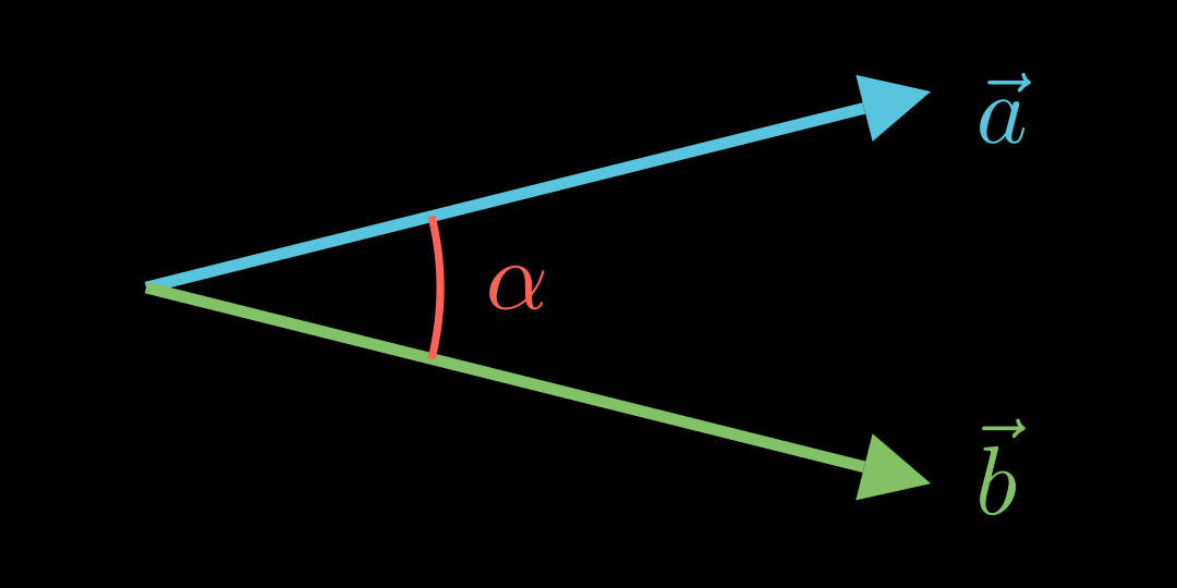
Winkel zwischen Vektoren 💡
Für den Winkel α \alpha α a ⃗ \vec a a b ⃗ \vec b b
cos ( α ) = a ⃗ ∘ b ⃗ ∣ a ⃗ ∣ ⋅ ∣ b ⃗ ∣ \cos(\alpha)=\frac{
\vec a \circ \vec b
}{
|\vec a| \cdot |\vec b|} cos ( α ) = ∣ a ∣ ⋅ ∣ b ∣ a ∘ b Beispiel a ⃗ = ( − 2 3 1 ) b ⃗ = ( 4 0 3 ) \vec a =
\left(\begin{matrix}
-2 \\ 3 \\ 1
\end{matrix}\right)
\qquad
\vec b =
\left(\begin{matrix}
4 \\ 0 \\ 3
\end{matrix}\right) a = − 2 3 1 b = 4 0 3 ∣ a ⃗ ∣ = 14 ∣ b ⃗ ∣ = 5 cos ( α ) = ( − 2 3 1 ) ∘ ( 4 0 3 ) 14 ⋅ 5 cos ( α ) = − 5 14 ⋅ 5 α = cos − 1 ( − 1 14 ) ⏟ DEGREE! ≈ 105 , 5 ° |\vec a| = \sqrt{14}
\qquad
|\vec b| = 5
\\
\begin{align*}
\\
\cos(\alpha) &= \frac{
\left(\begin{matrix}
-2 \\ 3 \\ 1
\end{matrix}\right)
\circ
\left(\begin{matrix}
4 \\ 0 \\ 3
\end{matrix}\right)
}{
\sqrt{14} \cdot 5
}
\\
\cos(\alpha) &= \frac{
-5}{
\sqrt{14} \cdot 5
}
\\
\alpha &=
\underbrace{
\cos^{-1}\left(-\frac{1}{\sqrt{14}}\right)
}_{
\color{red} \text{DEGREE!}
}
\boxed{\approx 105{,}5°}
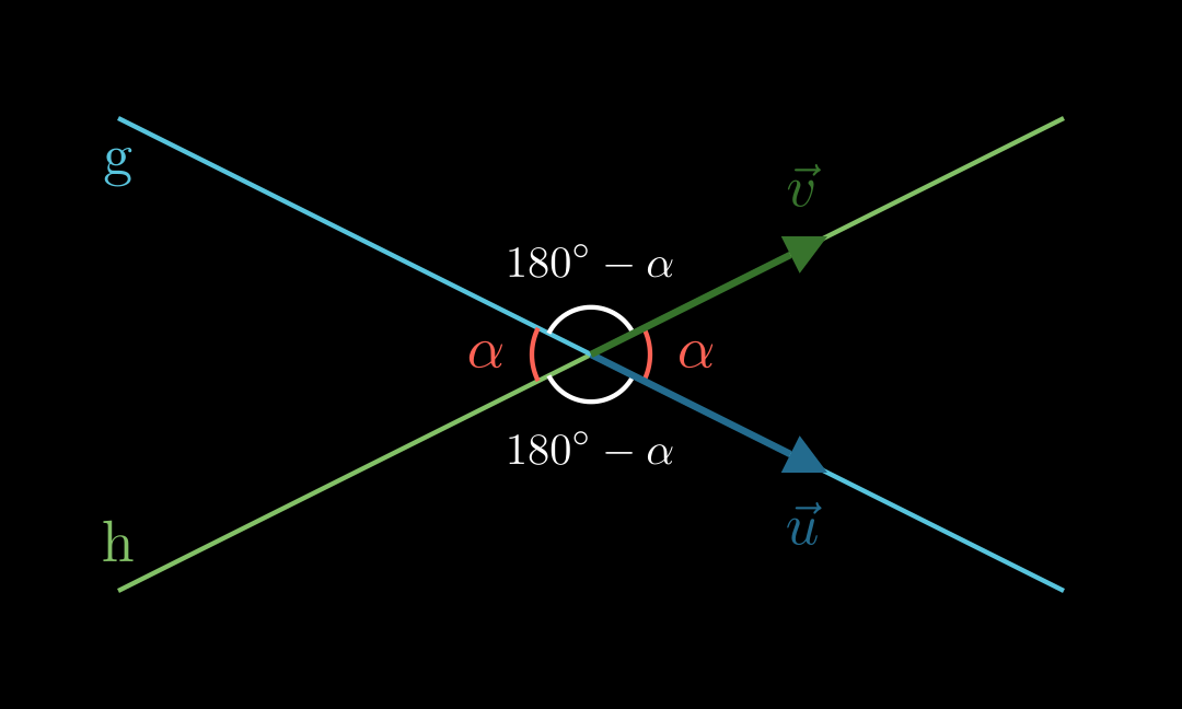
\end{align*} ∣ a ∣ = 14 ∣ b ∣ = 5 cos ( α ) cos ( α ) α = 14 ⋅ 5 − 2 3 1 ∘ 4 0 3 = 14 ⋅ 5 − 5 = DEGREE! cos − 1 ( − 14 1 ) ≈ 105 , 5° Schnittwinkel Gerade-Gerade 💡
Für den Schnittwinkel zwischen zwei Geraden g g g h h h u ⃗ \vec u u v ⃗ \vec v v
cos ( α ) = ∣ u ⃗ ∘ v ⃗ ∣ ∣ u ⃗ ∣ ⋅ ∣ v ⃗ ∣ \cos(\alpha) = \frac{
|\vec u \circ \vec v|}{
|\vec u| \cdot |\vec v|} cos ( α ) = ∣ u ∣ ⋅ ∣ v ∣ ∣ u ∘ v ∣ Beispiel u ⃗ = ( − 2 3 1 ) v ⃗ = ( 4 0 3 ) \vec u =
\left(\begin{matrix}
-2 \\ 3 \\ 1
\end{matrix}\right)
\qquad
\vec v =
\left(\begin{matrix}
4 \\ 0 \\ 3
\end{matrix}\right) u = − 2 3 1 v = 4 0 3 ∣ u ⃗ ∣ = 14 ∣ v ⃗ ∣ = 5 cos ( α ) = ∣ ( − 2 3 1 ) ∘ ( 4 0 3 ) ∣ 14 ⋅ 5 cos ( α ) = ∣ − 5 ∣ 14 ⋅ 5 α = cos − 1 ( 1 14 ) ⏟ DEGREE! ≈ 74 , 5 ° |\vec u| = \sqrt{14}
\qquad
|\vec v| = 5
\\
\begin{align*}
\\
\cos(\alpha) &= \frac{
\left|
\left(\begin{matrix}
-2 \\ 3 \\ 1
\end{matrix}\right)
\circ
\left(\begin{matrix}
4 \\ 0 \\ 3
\end{matrix}\right)
\right|
}{
\sqrt{14} \cdot 5
}
\\
\cos(\alpha) &= \frac{
|-5|}{
\sqrt{14} \cdot 5
}
\\
\alpha &=
\underbrace{
\cos^{-1}\left(\frac{1}{\sqrt{14}}\right)
}_{
\color{red} \text{DEGREE!}
}
\boxed{\approx 74{,}5°}
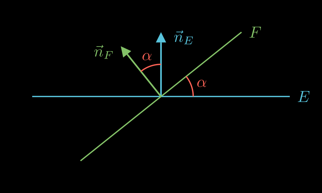
\end{align*} ∣ u ∣ = 14 ∣ v ∣ = 5 cos ( α ) cos ( α ) α = 14 ⋅ 5 − 2 3 1 ∘ 4 0 3 = 14 ⋅ 5 ∣ − 5∣ = DEGREE! cos − 1 ( 14 1 ) ≈ 74 , 5° Schnittwinkel Ebene-Ebene 💡
Für den Schnittwinkel zwischen zwei Ebenen E E E F F F n ⃗ E \vec n_E n E n ⃗ f \vec n_f n f
cos ( α ) = ∣ n ⃗ E ∘ n ⃗ F ∣ ∣ n ⃗ E ∣ ⋅ ∣ n ⃗ F ∣ \cos(\alpha) = \frac{
|\vec n_E \circ \vec n_F|}{
|\vec n_E| \cdot |\vec n_F|} cos ( α ) = ∣ n E ∣ ⋅ ∣ n F ∣ ∣ n E ∘ n F ∣ Beispiel Siehe Beispiel Schnittwinkel Gerade-Gerade.
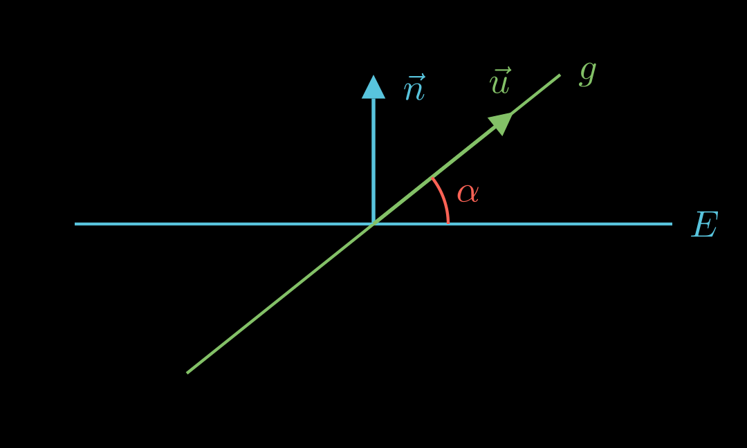
Schnittwinkel Gerade-Ebene 💡
Für den Schnittwinkel zwischen einer Geraden mit Richtungsvektoren u ⃗ \vec u u n ⃗ \vec n n
sin ( α ) = ∣ u ⃗ ∘ n ⃗ ∣ ∣ u ⃗ ∣ ⋅ ∣ n ⃗ ∣ {\color{red}\sin(\alpha)} = \frac{
|\vec u \circ \vec n|}{
|\vec u| \cdot |\vec n|} s i n ( α ) = ∣ u ∣ ⋅ ∣ n ∣ ∣ u ∘ n ∣ u ⃗ = ( 4 − 3 0 ) n ⃗ = ( 2 4 1 ) \vec u =
\left(\begin{matrix}
4 \\ -3 \\ 0
\end{matrix}\right)
\qquad
\vec n =
\left(\begin{matrix}
2 \\ 4 \\ 1
\end{matrix}\right) u = 4 − 3 0 n = 2 4 1 ∣ u ⃗ ∣ = 5 ∣ n ⃗ ∣ = 21 sin ( α ) = ∣ ( 4 − 3 0 ) ∘ ( 2 4 1 ) ∣ 5 ⋅ 21 sin ( α ) = ∣ − 4 ∣ 5 ⋅ 21 α = sin − 1 ( 4 5 ⋅ 21 ) ⏟ DEGREE! ≈ 10 , 1 ° |\vec u| = 5
\qquad
|\vec n| = \sqrt{21}
\\
\begin{align*}
\\
\sin(\alpha) &= \frac{
\left|
\left(\begin{matrix}
4 \\ -3 \\ 0
\end{matrix}\right)
\circ
\left(\begin{matrix}
2 \\ 4 \\ 1
\end{matrix}\right)
\right|
}{
5 \cdot \sqrt{21}
}
\\
\sin(\alpha) &= \frac{
|-4|}{
5 \cdot \sqrt{21}
}
\\
\alpha &=
\underbrace{
\sin^{-1}\left(\frac{4}{5 \cdot \sqrt{21}}\right)
}_{
\color{red} \text{DEGREE!}
}
\boxed{\approx 10{,}1°}
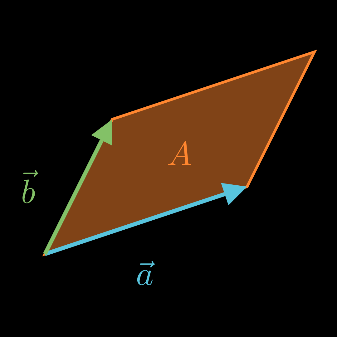
\end{align*} ∣ u ∣ = 5 ∣ n ∣ = 21 sin ( α ) sin ( α ) α = 5 ⋅ 21 4 − 3 0 ∘ 2 4 1 = 5 ⋅ 21 ∣ − 4∣ = DEGREE! sin − 1 ( 5 ⋅ 21 4 ) ≈ 10 , 1° Flächeninhalt Parallelogramm 💡
Für den Flächeninhalt A A A a ⃗ \vec a a b ⃗ \vec b b
A = ∣ a ⃗ × b ⃗ ∣ A=|\vec a \times \vec b| A = ∣ a × b ∣ Beispiel a ⃗ = ( 4 − 2 7 ) b ⃗ = ( 1 5 0 ) \vec a =
\left(\begin{matrix}
4 \\ -2 \\ 7
\end{matrix}\right)
\qquad
\vec b =
\left(\begin{matrix}
1 \\ 5 \\ 0
\end{matrix}\right) a = 4 − 2 7 b = 1 5 0 A = ∣ ( 4 − 2 7 ) × ( 1 5 0 ) ∣ = ∣ ( − 35 7 22 ) ∣ ≈ 41 , 93 A = \left|
\left(\begin{matrix}
4 \\ -2 \\ 7
\end{matrix}\right)
\times
\left(\begin{matrix}
1 \\ 5 \\ 0
\end{matrix}\right)
\right|
=
\left|
\left(\begin{matrix}
-35 \\ 7 \\ 22
\end{matrix}\right)
\right|
\approx
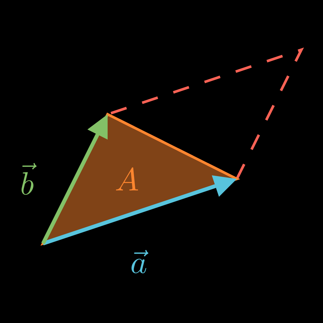
41{,}93 A = 4 − 2 7 × 1 5 0 = − 35 7 22 ≈ 41 , 93 Flächeninhalt Dreieck 💡
Für den Flächeninhalt A A A a ⃗ \vec a a b ⃗ \vec b b
A = 1 2 ⋅ ∣ a ⃗ × b ⃗ ∣ A = \frac12 \cdot
|\vec a \times \vec b| A = 2 1 ⋅ ∣ a × b ∣ Beispiel a ⃗ = ( 4 − 2 7 ) b ⃗ = ( 1 5 0 ) \vec a =
\left(\begin{matrix}
4 \\ -2 \\ 7
\end{matrix}\right)
\qquad
\vec b =
\left(\begin{matrix}
1 \\ 5 \\ 0
\end{matrix}\right) a = 4 − 2 7 b = 1 5 0 A = 1 2 ⋅ ∣ ( 4 − 2 7 ) × ( 1 5 0 ) ∣ = 1 2 ⋅ ∣ ( − 35 7 22 ) ∣ ≈ 1 2 ⋅ 41 , 93 = 20 , 965 A =
\frac12 \cdot
\left|
\left(\begin{matrix}
4 \\ -2 \\ 7
\end{matrix}\right)
\times
\left(\begin{matrix}
1 \\ 5 \\ 0
\end{matrix}\right)
\right|
=
\frac12 \cdot
\left|
\left(\begin{matrix}
-35 \\ 7 \\ 22
\end{matrix}\right)
\right|
\approx
\frac12 \cdot
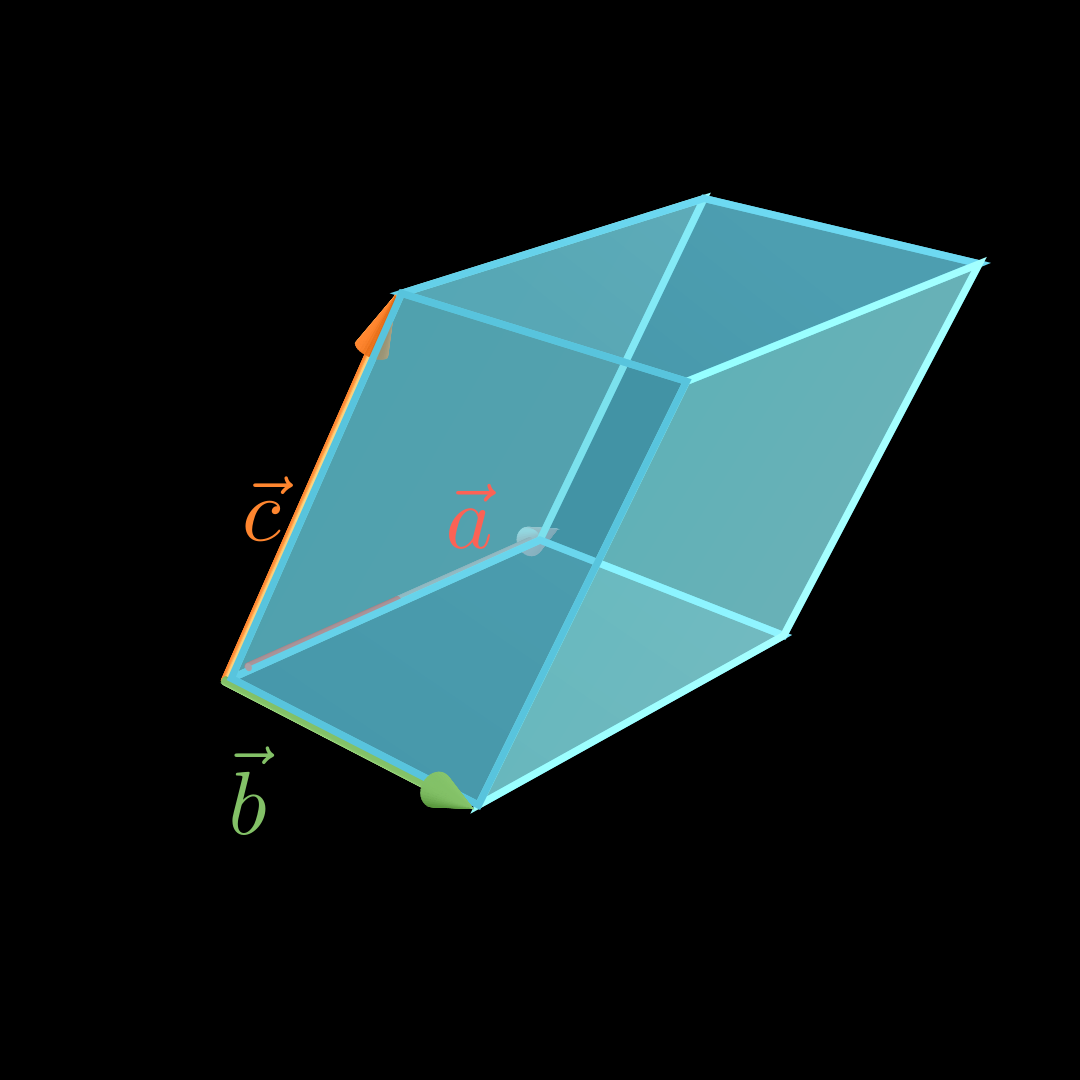
41{,}93 = 20{,}965 A = 2 1 ⋅ 4 − 2 7 × 1 5 0 = 2 1 ⋅ − 35 7 22 ≈ 2 1 ⋅ 41 , 93 = 20 , 965 Volumen Spat 💡
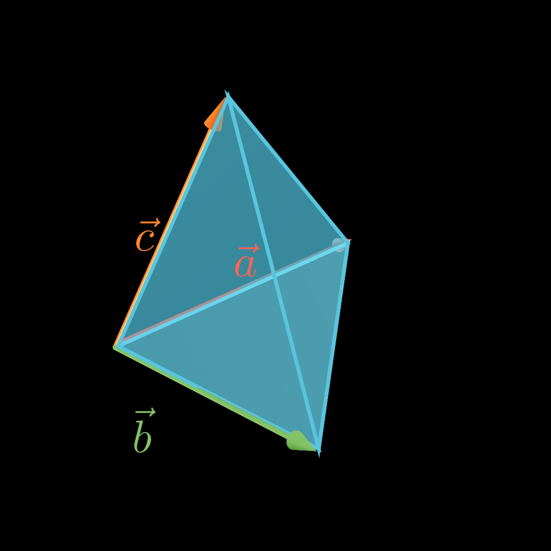
Für das Volumen V V V a ⃗ , b ⃗ \vec a, \vec b a , b c ⃗ \vec c c
V = ∣ ( a ⃗ × b ⃗ ) ∘ c ⃗ ∣ V =
|(\vec a \times \vec b)
\circ \vec c \, | V = ∣ ( a × b ) ∘ c ∣ Beispiel a ⃗ = ( − 4 2 0 ) b ⃗ = ( − 4 − 3 5 ) c ⃗ = ( − 2 0 10 ) \vec a =
\left(\begin{matrix}
-4 \\ 2 \\ 0
\end{matrix}\right)
\qquad
\vec b =
\left(\begin{matrix}
-4 \\ -3 \\ 5
\end{matrix}\right)
\qquad
\vec c =
\left(\begin{matrix}
-2 \\ 0 \\ 10
\end{matrix}\right) a = − 4 2 0 b = − 4 − 3 5 c = − 2 0 10 V = ∣ [ ( − 4 2 0 ) × ( − 4 − 3 5 ) ] ∘ ( − 2 0 10 ) ∣ = ∣ ( 10 20 20 ) ∘ ( − 2 0 10 ) ∣ = ∣ − 20 + 200 ∣ = 180 \begin{align*}
V &= \left|
\left[
\left(\begin{matrix}
-4 \\ 2 \\ 0
\end{matrix}\right)
\times
\left(\begin{matrix}
-4 \\ -3 \\ 5
\end{matrix}\right)
\right]
\circ
\left(\begin{matrix}
-2 \\ 0 \\ 10
\end{matrix}\right)
\right|
\\
&= \left|
\left(\begin{matrix}
10 \\ 20 \\ 20
\end{matrix}\right)
\circ
\left(\begin{matrix}
-2 \\ 0 \\ 10
\end{matrix}\right)
\right|
\\&=|{-20}+200|
\\&= 180
\end{align*} V = − 4 2 0 × − 4 − 3 5 ∘ − 2 0 10 = 10 20 20 ∘ − 2 0 10 = ∣ − 20 + 200∣ = 180 Volumen Pyramide mit viereckiger Grundfläche 💡
Für das Volumen V V V a ⃗ , b ⃗ \vec a, \vec b a , b c ⃗ \vec c c
V = 1 3 ⋅ ∣ ( a ⃗ × b ⃗ ) ∘ c ⃗ ∣ V = \frac13\cdot
|(\vec a \times \vec b)
\circ \vec c \, | V = 3 1 ⋅ ∣ ( a × b ) ∘ c ∣ Beispiel a ⃗ = ( − 4 2 0 ) b ⃗ = ( − 4 − 3 5 ) c ⃗ = ( − 2 0 10 ) \vec a =
\left(\begin{matrix}
-4 \\ 2 \\ 0
\end{matrix}\right)
\qquad
\vec b =
\left(\begin{matrix}
-4 \\ -3 \\ 5
\end{matrix}\right)
\qquad
\vec c =
\left(\begin{matrix}
-2 \\ 0 \\ 10
\end{matrix}\right) a = − 4 2 0 b = − 4 − 3 5 c = − 2 0 10 V = 1 3 ⋅ ∣ [ ( − 4 2 0 ) × ( − 4 − 3 5 ) ] ∘ ( − 2 0 10 ) ∣ = 1 3 ⋅ ∣ ( 10 20 20 ) ∘ ( − 2 0 10 ) ∣ = 1 3 ⋅ ∣ − 20 + 200 ∣ = 1 3 ⋅ 180 = 60 \begin{align*}
V &= \frac13 \cdot
\left|
\left[
\left(\begin{matrix}
-4 \\ 2 \\ 0
\end{matrix}\right)
\times
\left(\begin{matrix}
-4 \\ -3 \\ 5
\end{matrix}\right)
\right]
\circ
\left(\begin{matrix}
-2 \\ 0 \\ 10
\end{matrix}\right)
\right|
\\
&= \frac13 \cdot
\left|
\left(\begin{matrix}
10 \\ 20 \\ 20
\end{matrix}\right)
\circ
\left(\begin{matrix}
-2 \\ 0 \\ 10
\end{matrix}\right)
\right|
\\&=\frac13 \cdot|{-20}+200|
\\&=\frac13 \cdot 180
\\&= 60
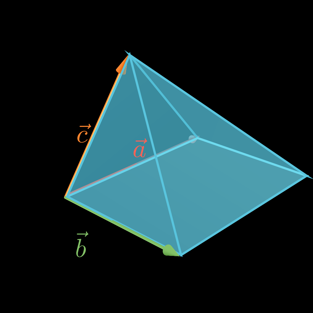
\end{align*} V = 3 1 ⋅ − 4 2 0 × − 4 − 3 5 ∘ − 2 0 10 = 3 1 ⋅ 10 20 20 ∘ − 2 0 10 = 3 1 ⋅ ∣ − 20 + 200∣ = 3 1 ⋅ 180 = 60 Volumen Pyramide mit dreieckiger Grundfläche 💡
Für das Volumen V V V a ⃗ , b ⃗ \vec a, \vec b a , b c ⃗ \vec c c
V = 1 6 ⋅ ∣ ( a ⃗ × b ⃗ ) ∘ c ⃗ ∣ V = \frac16\cdot
|(\vec a \times \vec b)
\circ \vec c \, | V = 6 1 ⋅ ∣ ( a × b ) ∘ c ∣ Beispiel a ⃗ = ( − 4 2 0 ) b ⃗ = ( − 4 − 3 5 ) c ⃗ = ( − 2 0 10 ) \vec a =
\left(\begin{matrix}
-4 \\ 2 \\ 0
\end{matrix}\right)
\qquad
\vec b =
\left(\begin{matrix}
-4 \\ -3 \\ 5
\end{matrix}\right)
\qquad
\vec c =
\left(\begin{matrix}
-2 \\ 0 \\ 10
\end{matrix}\right) a = − 4 2 0 b = − 4 − 3 5 c = − 2 0 10 V = 1 6 ⋅ ∣ [ ( − 4 2 0 ) × ( − 4 − 3 5 ) ] ∘ ( − 2 0 10 ) ∣ = 1 6 ⋅ ∣ ( 10 20 20 ) ∘ ( − 2 0 10 ) ∣ = 1 6 ⋅ ∣ − 20 + 200 ∣ = 1 6 ⋅ 180 = 30 \begin{align*}
V &= \frac16 \cdot
\left|
\left[
\left(\begin{matrix}
-4 \\ 2 \\ 0
\end{matrix}\right)
\times
\left(\begin{matrix}
-4 \\ -3 \\ 5
\end{matrix}\right)
\right]
\circ
\left(\begin{matrix}
-2 \\ 0 \\ 10
\end{matrix}\right)
\right|
\\
&= \frac16 \cdot
\left|
\left(\begin{matrix}
10 \\ 20 \\ 20
\end{matrix}\right)
\circ
\left(\begin{matrix}
-2 \\ 0 \\ 10
\end{matrix}\right)
\right|
\\&=\frac16 \cdot|{-20}+200|
\\&=\frac16 \cdot 180
\\&= 30
\end{align*} V = 6 1 ⋅ − 4 2 0 × − 4 − 3 5 ∘ − 2 0 10 = 6 1 ⋅ 10 20 20 ∘ − 2 0 10 = 6 1 ⋅ ∣ − 20 + 200∣ = 6 1 ⋅ 180 = 30 Spiegelung
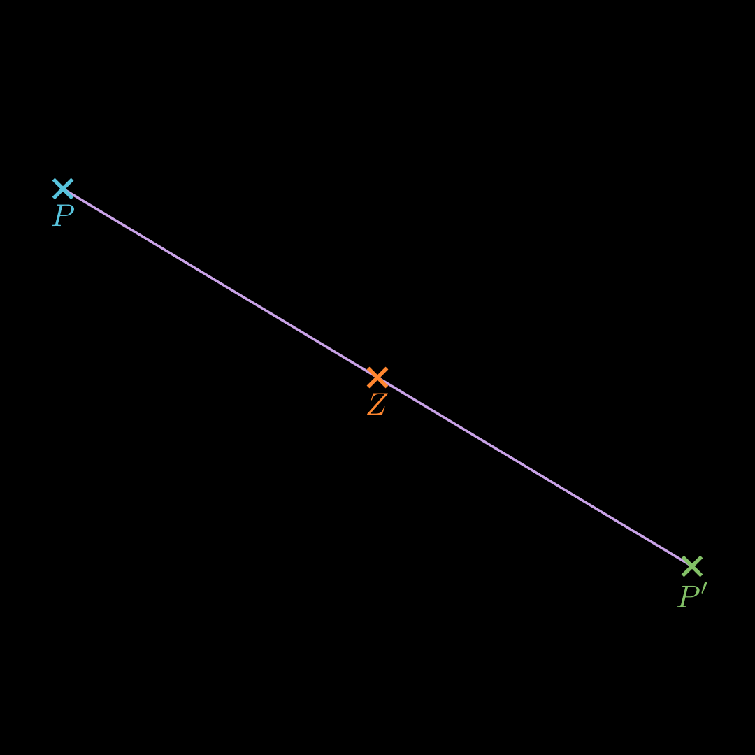
An einem Punkt spiegeln 💡
O P ′ → = O P → + 2 ⋅ P Z → = O Z → + P Z → \begin{align*}
\overrightarrow{OP'} &=
\overrightarrow{OP} + 2 \cdot \overrightarrow{PZ}\\
&=
\overrightarrow{OZ} +
\overrightarrow{PZ}
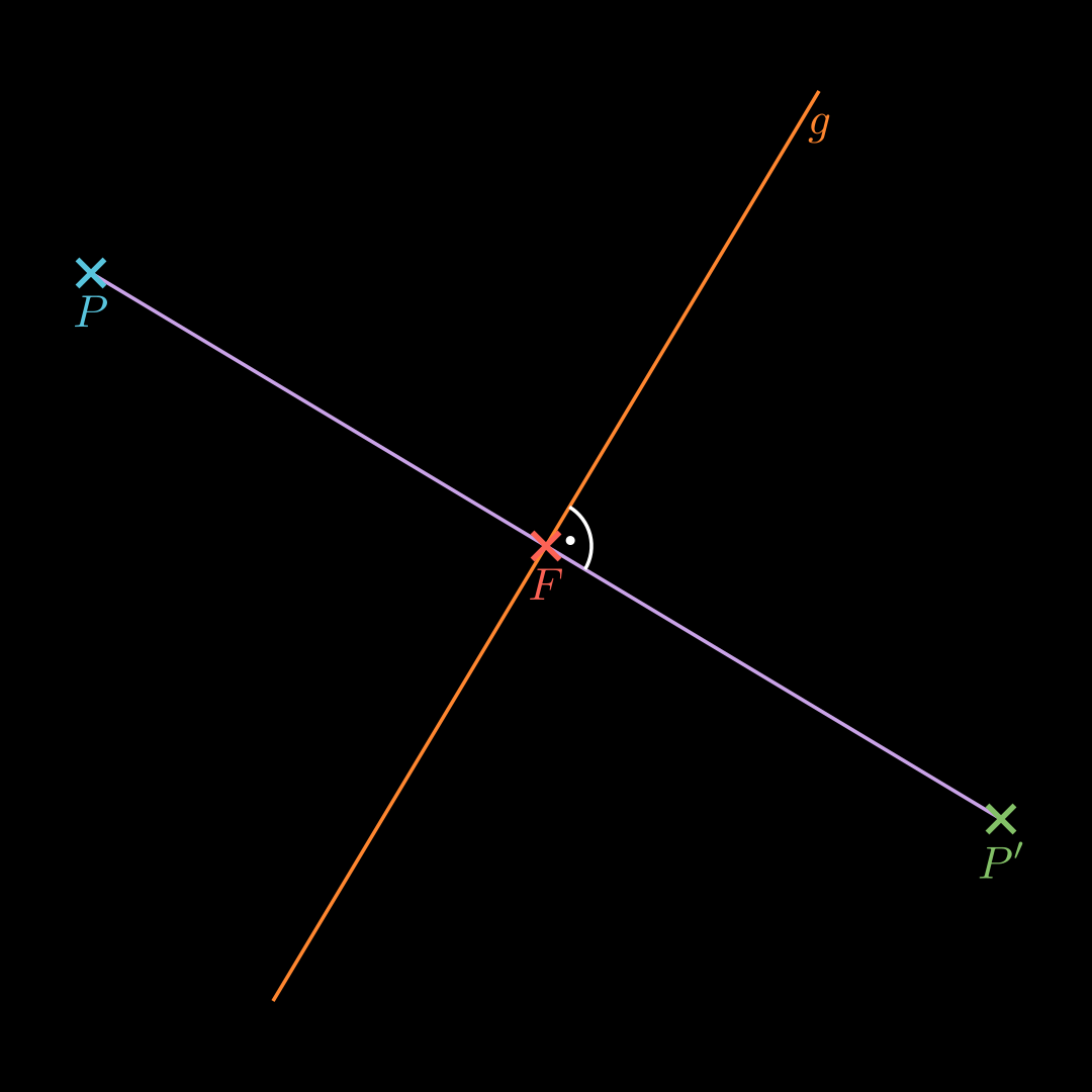
\end{align*} O P ′ = OP + 2 ⋅ PZ = OZ + PZ An einer Geraden spiegeln 💡
Stelle eine Hilfsebene H H H P P P g g g Erhalte den Punkt F F F g g g H H H Punktspiegelung an F F F O P ′ → = O F → + P F → \overrightarrow{OP'} = \overrightarrow{OF} + \overrightarrow{PF} O P ′ = OF + PF An einer Ebene Spiegeln 💡
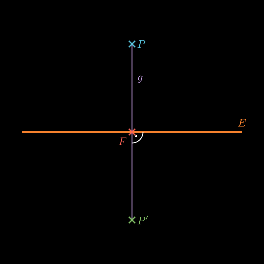
Stelle eine Gerade g g g E E E P P P Erhalte den Punkt F F F g g g E E E Punktspiegelung an F F F O P ′ → = O F → + P F → \overrightarrow{OP'} = \overrightarrow{OF} + \overrightarrow{PF} O P ′ = OF + PF Symmetrieebene bestimmen 💡
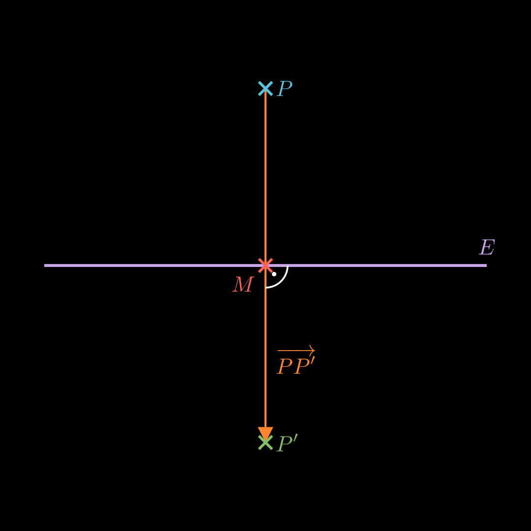
Berechne den Mittelpunkt M M M P P P P ’ P’ P ’ Stelle eine Gleichung für E E E M M M E E E P P ′ → \overrightarrow{PP'} P P ′ E E E
🔎